
The spread of disease, politics, the movement of animals, regions vulnerable to earthquakes and where people are most likely to buy frosted flakes are all informed by spatial data. Spatial data links information to specific positions on earth and can tell us about patterns that play out from location to location. We can use spatial data to uncover processes over space and tackle complex problems.
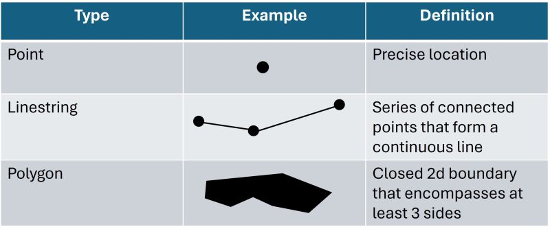
Spatial data, or information on the geographic position of things, can be represented in different ways. For instance, if you’re meeting a friend for coffee and have her exact location, this is an example of point data. Point data is a specific coordinate, or individual point, allowing you to identify the precise location of something. Now consider wanting to find a Virginia state forest to visit, including all its features within a specific boundary. This scenario exemplifies polygon data, representing a region enclosed by a defined boundary. Similarly, trails and rivers within the forest boundary can be represented as linestrings or connected line segments. All situations involve location-based information, but they are represented in various ways. In this article, we will explore and work with three types of spatial data, (a) points, (b) linestrings, and (c) polygons.
Suppose you and your friend forgo the forests and decide to explore coffee shops in a few cities. To decide where and what coffee shops to visit you need to know two things: (a) the boundary defining where cities are, and (b) the location of coffee shops in these cities.
We can combine these pieces of information to get a map of coffee shops in cities by overlaying the coffee shop locations onto the city outline. Each unique dataset is called a layer. Multiple layers can be combined or ‘stacked’ on top of each other to represent various geographic pieces on information on a single map. Our analysis or map can incorporate multiple layers, allowing us to include different sources of spatial information.
Working with spatial data
Working with spatial data in R is easy! In this article, we’ll be using the Simple Features for R package, also known as the sf package which makes it straightforward to manipulate and analyze spatial data. If you do not have the sf or any another package, you can install it using the install.packages() function. After installing these packages, you can load them for each R session using library() as we will do here. Let’s go ahead and load the various R packages we’ll use in this article.
library(sf)          #For working with spatial data
library(tidyverse)   #For data wrangling and ggplot2
library(ggspatial)   #For spatial data with ggplot2
library(tigris)      #For downloading spatial data directly into R
You love cities and recently moved to Charlottesville, Virginia, for school but you’re excited to explore all the places Virginia has to offer. However, you can’t find a map that provides all the information you want, so you need to use spatial information to build your own map to help you navigate around. Let’s start by reading in our first layer, the boundary or shape of Virginia. This layer is a polygon and it is contained in a shapefile. A shapefile is simply a format type for storing geographic data and has a .shp extension. A shapefile is part of a network of multiple files that all work together, so it’s important to store them in the same folder. Click here to download the Virginia spatial files used in this article if you would like to follow along.
We will read in a shapefile of a Virginia polygon using st_read() and check the geometry type by calling st_geometry_type() on our spatial data. Checking the geometry will tell us the type of spatial data we are working with (ex. point, linestring). The polygon we will use for Virginia is from the Virginia Department of Emergency Management.
#Read in Virginia polygon
virginia <- st_read("VirginiaBoundary.shp")
#Check geometry type
as.character(st_geometry_type(virginia))[1]
[1] "POLYGON"
We can take a look at our Virginia boundary by calling the plot() function on our spatial data. We need to tell R to specifically plot the geometry column that contains the spatial data, otherwise, R will plot the Virginia boundary for every column in our data frame.
plot(virginia$geometry)
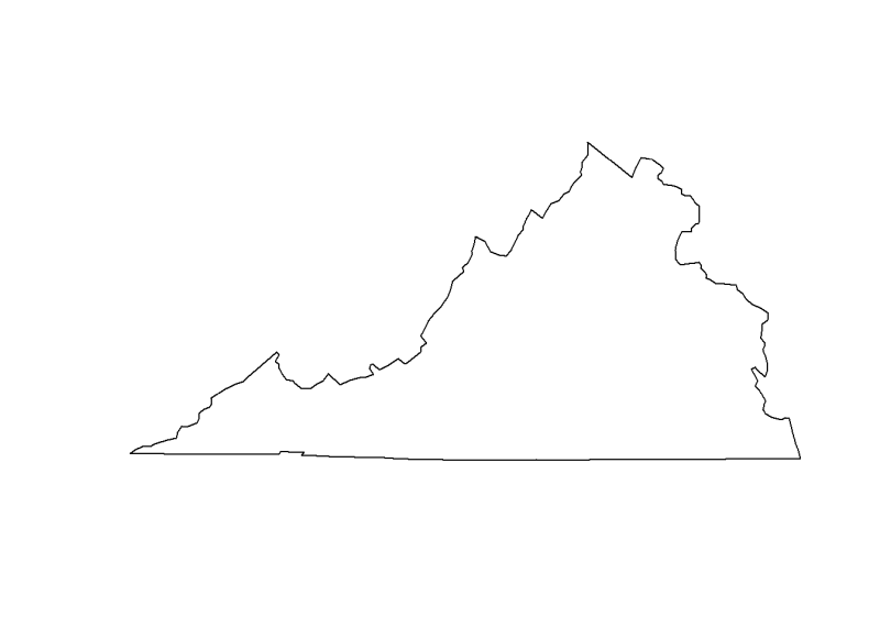
Great! We have the outline of Virginia. Let’s add our city locations by making a data frame with the cities that we are interested in visiting. We will take a look at the structure of this data frame using str().
#Data frame of cities
cities <- data.frame(
  City = c("Richmond", "Virginia Beach", "Norfolk", "Chesapeake", "Arlington", "Charlottesville"),
  Latitude = c(37.5413, 36.8529, 36.8508, 36.7682, 38.8797, 38.0293),
  Longitude = c(-77.4348, -75.9780, -76.2859, -76.2875, -77.1080, -78.4767))
#Examine structure of data frame
str(cities)
'data.frame':   6 obs. of  3 variables:
 $ City     : chr  "Richmond" "Virginia Beach" "Norfolk" "Chesapeake" ...
 $ Latitude : num  37.5 36.9 36.9 36.8 38.9 ...
 $ Longitude: num  -77.4 -76 -76.3 -76.3 -77.1 ...
We can see that our data frame has 6 observations of 3 variables or columns. In our data frame, we have a column for the city name, as well as the latitude and longitude of the city. The latitude and longitude columns define our coordinates and provide locations of these places on earth. Notably, our cities are characters while our latitude and longitude are numeric values. But, how does R know these numbers should represent locations? To tell R this data is spatial information, we are going to convert these values to a column that contains a geometry. Like our polygon of Virginia, our geometry column contains the data structure to represent spatial features. To do this conversion, we will use the function st_as_sf() from the sf package. We will input the data frame to use, the columns to convert to a geometry (our Latitude and Longitude columns) and also tell R to not remove the original Longitude and Latitude columns by setting the argument remove = FALSE. You can choose to remove the numeric Longitude and Latitude columns from the data frame by leaving this argument out or setting it to TRUE, which is the default. We will also start by setting crs = 4326, a common global system to reference our locations. We will review the crs argument in the next section.
#Convert to sf object
cities.sf <-
  st_as_sf(cities, coords = c("Longitude", "Latitude"), remove = FALSE, crs = 4326)
#Plot the cities
plot(cities.sf$geometry)
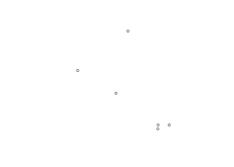
When we work with data frames containing latitude and longitude information, we have the opportunity to understand the spatial context of the data. Keep in mind that these latitude and longitude coordinates are point data representing specific locations on earth. However, looking at the city points alone doesn’t give us the spatial context we need, so lets add the Virginia boundary as a layer. Before we can put these 2 layers together, we need to look at how our data is represented because we can measure spatial data in different ways.
We will check this by calling st_crs() from the sf package to get the structure of our spatial data. This function will give us information on the coordinate reference system (CRS), which we will explore in the next section.
st_crs(virginia)$epsg
[1] 4269
st_crs(cities.sf)$epsg
[1] 4326
Essentially, the way we have represented our layers are different. What does this mean and how can we fix it?
Defining spatial data
Imagine you are now working in a coffee shop and the manager asks you to measure the bar length so they can order a new one since this bar has gotten old. You tell your manager it is four. 4 feet? 4 meters? Certainly it can’t be very small coming in at 4 cm or very large at 4 miles! If it is truly 4 feet, we can say it is also 1.2 meters (4 ft = 1.2 m) while if it is actually 4 meters, the bar is longer at 13 feet and can probably fit a few more people. Both of these options seem reasonable to the manager since they have not been into the shop before, but which is it? It certainly can’t be both since the length of the bar hasn’t changed, but rather the unit of measuring the bar has.
Similarly, we have different ways to present the spatial information associated with our data. We will explore ways to show our data by going over two important components of spatial data: (a) datums and (b) projections. We’ll also cover how to represent them using (a) coordinate reference systems and (b) EPSG codes.
Remember that coordinates are a pair of numbers that tell us the location of something. A datum specifies the frame for our coordinates. This means that a datum provides the foundation for defining where things are relative to one another. In other words, it tells us the “origin and orientation of latitude and longitude lines” (esri, Datums). Coordinates are associated with units (ex. meters, degrees) and are also different for different datums, so defining the correct datum is important!
Phew! We can represent locations on earth now and have identified a means to do so. But, we still face a challenge - the earth isn’t flat. It’s a sphere which is 3-dimensional while we want to create a map that is only 2-dimensional. We can manage this problem by setting a projection. Defining a projection allows us to represent something that is 3-dimensional on a 2-dimensional plane. Essentially, a projection tells us how the 3-dimensional space will be projected, or drawn, onto a 2-dimensional surface.
So, the datum gives us a reference frame for the location of things while the projection tells us how to draw them on a flat surface. We can tie these components together by using a CRS (coordinate reference system). A CRS offers a standardized method to define locations and can be referenced by an EPSG code which is a unique identifier for geographic objects. You can find more on EPSG codes by visiting this website. We need our CRS to be consistent across all layers so that they align properly. If the CRS is different, you will likely encounter an error in R, indicating that the CRS of layer1 doesn’t match the CRS of layer2.
Now that we know about the structure of our spatial data, we need to ensure our Virginia polygon and city points have the same CRS. We will do this by calling st_transform() on our data. This sf function will take our spatial data and transform it to the CRS we set. We will use the EPSG 26918 which is a projected coordinate system commonly used in North America. We will then check that our layers have the same CRS by seeing if the CRS of virginia.crs is equal to (==) the CRS of cities.crs.
#Transform CRS
virginia.crs <- st_transform(virginia, crs = 26918)
cities.crs <- st_transform(cities.sf, crs = 26918)
#Check that the layers have the same CRS
st_crs(virginia.crs) == st_crs(cities.crs)
[1] TRUE
If you run into further issues or want to explore the data more, you can also troubleshoot by checking the coordinate values by calling head(st_coordinates(df)) on your data frame.
Plotting with ggplot
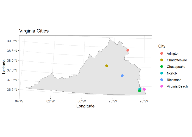
Now that we’ve brought in our data, converted it to a spatial object, and made sure our layers align, let’s create our map. We’ll use ggplot() and call geom_sf() which tells R that we’re working with spatial data. When making a map, it’s also crucial to consider the order of our layers. If we place our cities data (cities.crs) before the Virginia polygon (virginia.crs), the cities will end up under the Virginia polygon and we won’t be able to see them.
ggplot() +
  #Add Virginia polygon
  geom_sf(data = virginia.crs) +
  #Add cities layer
  geom_sf(data = cities.crs, aes(color = City, label = City), size = 3) +
  #Add titles
  labs(x = "Longitude", y = "Latitude", title = "Virginia Cities") +
  #Add theme
  theme_bw()
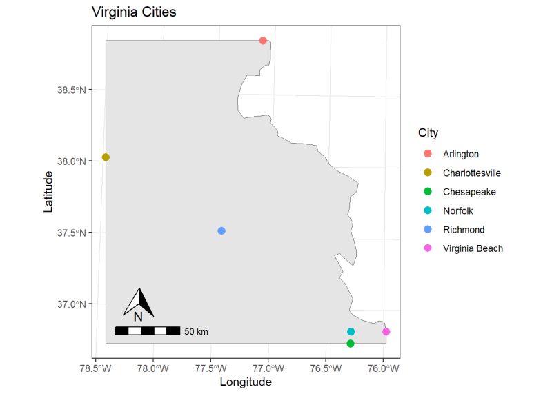
Since the cities we want to visit are in the eastern region of the state, we’ll ‘zoom in’ on this area by defining a bounding box around our cities. A bounding box defines a rectangle that encompasses the extent of our features of interest. We will get our bounding box of the cities extent and crop virginia.crs to this region by calling st_crop().
#Get bounding box of the cities
cities.extent <- st_bbox(cities.crs)
Additionally, we’ll add some custom elements to our map, like a north arrow and a scale bar, using the ggspatial R package.
#Plot using the packages ggplot and ggspatial
ggplot() +
  #Crop Virginia boundary to spatial extent of cities and add Virginia layer
  geom_sf(data = st_crop(virginia.crs, cities.extent)) +
  #Add cities layer
  geom_sf(data = cities.crs, aes(color = City, label = City), size = 3) +
  #Add scale bar to bottom left from ggspatial
  annotation_scale(location = "bl", height = unit(.25, "cm"),
                   width = unit(1, "cm"), pad_x = unit(0.3, "in"),
                   pad_y = unit(0.3, "in")) +
  #Add north arrow to bottom left from ggspatial
  annotation_north_arrow(height = unit(1, "cm"), width = unit(1, "cm"),
                         which_north = "true", location = "bl",
                         pad_x = unit(0.4, "in"), pad_y = unit(0.5, "in")) +
  #Add titles
  labs(x = "Longitude", y = "Latitude", title = "Virginia Cities") +
  #Add theme
  theme_bw()
Extracting information in spatial data
There is still a lot of information we can gather from this data outside of the map itself! How far from the Virginia border are the cities? What is the distance from each city to Charlottesville? What is the area of each city that we can explore? Answering these questions is easy using sf! We will first get the distance from each city to the border using the st_distance() function on the boundary of the Virginia polygon (st_boundary()). The st_distance() function calculates the distance between two spatial objects. Here, we calculate the Euclidean distance, or the shortest distance between two spatial objects.
#Distance from each city to the border of Virginia
dist.border <-  st_distance(cities.crs, st_boundary(virginia.crs))
#See results
print(dist.border)
Units: [m]
           [,1]
[1,] 85469.5113
[2,]   121.7268
[3,] 11906.0329
[4,] 20091.7204
[5,]  3054.4664
[6,] 82565.9571
When we take a look at the distances, we see [m] at the top, indicating that these results are in the units of meters. If you would like to convert these values to a numeric class, you can do so using as.numeric() on the distance column, or you can add them to your data frame for later use by calling cities.crs$distance_to_border <- dist.border. From our results, we can see that Virginia Beach is closest to the Virginia border while Richmond is farthest.
However, we are in Charlottesville, and so we want how far each city is from Charlottesville. We calculate these distances and add them to our cities.crs data frame.
#Calculate distance from Charlottesville to each city
dist.cville <-
  st_distance(cities.crs, filter(cities.crs, City == "Charlottesville")) %>%
  bind_cols(cities.crs)
#Look at first 3 distances
head(dist.cville, n = 3)
Simple feature collection with 3 features and 4 fields
Geometry type: POINT
Dimension:     XY
Bounding box:  xmin: 284889.6 ymin: 4079001 xmax: 412812.9 ymax: 4157709
Projected CRS: NAD83 / UTM zone 18N
             .           City Latitude Longitude                 geometry
1 106615.8 [m]       Richmond  37.5413  -77.4348 POINT (284889.6 4157709)
2 256808.3 [m] Virginia Beach  36.8529  -75.9780 POINT (412812.9 4079001)
3 233902.9 [m]        Norfolk  36.8508  -76.2859 POINT (385359.8 4079093)
Since we’ve figured out how far these cities are from us, let’s now look at some navigation routes and the area of each city to estimate the size and the space available for us to explore. We will start by obtaining county data for Virginia using the tigris package, which provides access to geographic and spatial information from the U.S. Census Bureau. We’ll retrieve layers for the county boundaries (counties()) and primary roads (primary_roads()). Our road layer is a linestring or a sequence of continuous lines.
Keep in mind that it’s important to check the CRS of each layer and transform them if they do not match; otherwise, we’ll encounter errors when plotting the layers due to mismatched projections.
#Get county data for Virginia from tigris package and transform the CRS
va.counties <- counties(state = "VA") %>%
  st_transform(crs = 26918)
#Get road data and transform the CRS
roads <- primary_secondary_roads(state = "VA", year = 2021) %>% st_transform(crs = 26918)
#Plot with ggplot
ggplot() +
  #Crop Virginia counties to cities extent and plot
  geom_sf(data = st_crop(va.counties, cities.extent), color = "gray100", fill = "gray88", size = .25) +
  #Crop roads to cities extent and plot
  geom_sf(data = st_crop(roads, cities.extent), color = "black", size = .3) +
  #Plot cities
  geom_sf(data = cities.crs, aes(color = City), size = 4) +
  #Add titles
  labs(x = "Longitude", y = "Latitude", title = "Map of Virginia Cities") +
  #Adjust theme
  theme_bw() +
  theme(plot.title = element_text(hjust = 0.5))
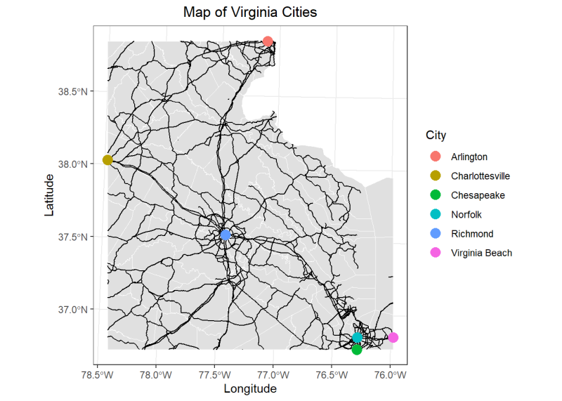
Now that we can visualize the boundary of each city and potential navigation routes to get there, we can calculate the area of our cities using st_area(). We will calculate the area for each of our 6 cities and create a column, area using mutate() to hold the calculated areas.
#Calculate area of each city we want to visit
county.area <- va.counties %>%
  select(NAME, geometry) %>%         #Select NAME and geometry columns
  filter(NAME %in% cities$City) %>%  #Filter to rows where NAME is in the City column of the cities data frame
  mutate(area = st_area(geometry))   #Create a column of areas using st_area()
#Output county name and area
county.area %>%
  select(NAME, area)
Simple feature collection with 7 features and 2 fields
Geometry type: MULTIPOLYGON
Dimension:     XY
Bounding box:  xmin: 190674 ymin: 4045325 xmax: 428626.1 ymax: 4311631
Projected CRS: NAD83 / UTM zone 18N
             NAME             area                       geometry
1 Charlottesville   26620749 [m^2] MULTIPOLYGON (((190676.7 42...
2        Richmond  162115691 [m^2] MULTIPOLYGON (((270200.2 41...
3      Chesapeake  908525938 [m^2] MULTIPOLYGON (((366512.5 40...
4       Arlington   67607783 [m^2] MULTIPOLYGON (((311606.8 43...
5         Norfolk  249559097 [m^2] MULTIPOLYGON (((380155.2 40...
6  Virginia Beach 1287748687 [m^2] MULTIPOLYGON (((390519.1 40...
7        Richmond  560255711 [m^2] MULTIPOLYGON (((358946.8 42...
Here, we can see the area of each city in \(m^2\). We can also see that the geometry type of our counties is a multipolygon, or a collection of polygons. This makes sense since each county that we have is a polygon shape, and we have multiple of them! We can also see the coordinates of our bounding box in Bounding box as well the CRS used. Remember, we can also get the spatial information by calling st_crs(df)$datum for the datum or st_crs(df)$proj for the projection.
st_crs(county.area)$datum
[1] "NAD83"
st_crs(county.area)$proj
[1] "utm"
We could easily convert our area values to square miles or square kilometers by applying the correct conversion factor, if needed.
Conclusion
We’ve explored different types of spatial data, ensured proper formatting, and covered several techniques for visualization and data analysis. However, the ability to use spatial information does not end here! You can use distance or area as a predictor variable in a model, visualize income by city on a map, or simply plot your latitude and longitude points for a simple representation of your data locations. You can join datasets based on geographic features (st_join()), find where features intersect (st_intersects()), or even do geospatial statistics. There are also opportunities to use many layers or data sources and include different spatial data types, like we’ve done here by including point, linestring, and polygon data.
To further explore the sf package, check out this R spatial github, and if you’re interested in creating interactive maps, check out our article Data Scientist as Cartographer: An Introduction to Making Interactive Maps in R with Leaflet!
R session details
The analysis was done using the R Statistical language (v4.5.1; R Core Team, 2025) on Windows 11 x64, using the packages ggspatial (v1.1.9), lubridate (v1.9.4), tibble (v3.3.0), sf (v1.0.21), tigris (v2.2.1), ggplot2 (v3.5.2), forcats (v1.0.0), stringr (v1.5.1), tidyverse (v2.0.0), dplyr (v1.1.4), purrr (v1.1.0), readr (v2.1.5) and tidyr (v1.3.1).
References
- Dunnington, D. (2023). ggspatial: Spatial Data Framework for ggplot2. R package version 1.1.9, https://CRAN.R-project.org/package=ggspatial.
- Esri https://desktop.arcgis.com/en/arcmap/latest/map/projections/datums.htm
- Pebesma, E., & Bivand, R. (2023). Spatial Data Science: With Applications in R. Chapman and Hall/CRC. https://doi.org/10.1201/9780429459016
- R Core Team (2024). R: A Language and Environment for Statistical Computing. R Foundation for Statistical Computing, Vienna, Austria. https://www.R-project.org/.
- Virginia Department of Emergency Management (2024). https://vgin.vdem.virginia.gov/datasets/777890ecdb634d18a02eec604db522c6/about.
- Walker, K. (2023). tigris: Load Census TIGER/Line Shapefiles. R package version 2.0.4, https://CRAN.R-project.org/package=tigris.
- Wickham, H., Averick, M., Bryan, J., Chang, W., McGowan, LD., François, R., Grolemund, G., Hayes, A., Henry, L., Hester, J., Kuhn, M., Pedersen, TL., Miller, E., Bache, SM., Müller, K., Ooms, J., Robinson, D., Seidel, DP., Spinu, V., Takahashi, K., …Yutani, H. (2019). “Welcome to the tidyverse.” Journal of Open Source Software, 4(43), 1686. doi:10.21105/joss.01686 https://doi.org/10.21105/joss.01686.
Lauren Brideau
StatLab Associate
University of Virginia Library
May 16, 2024
For questions or clarifications regarding this article, contact statlab@virginia.edu.
View the entire collection of UVA Library StatLab articles, or learn how to cite.