
Generalized estimating equations, or GEE, is a method for modeling longitudinal or clustered data. It is usually used with non-normal data such as binary or count data. The name refers to a set of equations that are solved to obtain parameter estimates (i.e., model coefficients). If interested, see Agresti (2002) for the computational details. In this article we simply aim to get you started with implementing and interpreting GEE using the R statistical computing environment.
We often model longitudinal or clustered data with mixed-effect or multilevel models. So how is GEE different?
- The main difference is that it’s a marginal model. It seeks to model a population average. Mixed-effect/multilevel models are subject-specific, or conditional, models. They allow us to estimate different parameters for each subject or cluster. In other words, the parameter estimates are conditional on the subject/cluster. This in turn provides insight to the variability between subjects or clusters. We can also obtain a population-level model from a mixed-effect model, but it’s basically an average of the subject-specific models.
- GEE is intended for simple clustering or repeated measures. It cannot easily accommodate more complex designs such as nested or crossed groups; for example, nested repeated measures within a subject or group. This is something better suited for a mixed-effect model.
- GEE computations are usually easier than mixed-effect model computations. GEE does not use the likelihood methods that mixed-effect models employ, which means GEE can sometimes estimate more complex models.
- Because GEE doesn’t use likelihood methods, the estimated “model” is incomplete and not suitable for simulation.
- GEE allows us to specify a correlation structure for different responses within a subject or group. For example, we can specify that the correlation of measurements taken closer together is higher than those taken farther apart. This is not something that’s currently possible in the popular lme4 package.
Let’s work through an example to compare and contrast GEEs and mixed-effect models. The data we’ll use come from Table 11.2 of Agresti (2002) and concern a longitudinal study comparing two drugs (“new” versus “standard”) for treating depression. Below we read in the data from a .csv file, set “standard” as the reference level for the drug variable, and look at the first three rows. We see subject 1 (id = 1) had a “mild” diagnosis and was treated with the “standard” drug at times 0, 1, and 2. At each time point, the subject’s depression response was a “1”, which in this case means “Normal”. A response of 0 means “Abnormal.”
URL <- "http://static.lib.virginia.edu/statlab/materials/data/depression.csv"
dat <- read.csv(URL, stringsAsFactors = TRUE)
dat$id <- factor(dat$id)
dat$drug <- relevel(dat$drug, ref = "standard")
head(dat, n = 3)
  diagnose     drug id time depression
1     mild standard  1    0          1
2     mild standard  1    1          1
3     mild standard  1    2          1
Altogether we have data on 340 subjects.
length(unique(dat$id))
[1] 340
Let’s look at the proportion of “Normal” responses (depression == 1) over time within the diagnosis and drug categories. Below we create a table of means by diagnosis, drug, and time. Recall that the mean of zeroes and ones is the proportion of ones. Then we “flatten” the table with ftable() and round the results to two digits using the pipe operator courtesy of the magrittr package. This reproduces Table 11.3 in Agresti (2002). Notice the proportion of “Normal” increases over time for all four combinations of diagnosis and treatment, and that the increase is more dramatic for the “new” drug.
library(magrittr)
with(dat, tapply(depression, list(diagnose, drug, time), mean)) %>%
  ftable() %>%
  round(2)
                    0    1    2

mild   standard  0.51 0.59 0.68
       new       0.53 0.79 0.97
severe standard  0.21 0.28 0.46
       new       0.18 0.50 0.83
Now let’s use GEE to estimate a marginal model for the effect of diagnosis, drug, and time on the depression response. We’ll also allow an interaction for drug and time. (This means we’re allowing the response trajectory to vary depending on drug.) We’ll use the gee() function in the gee package to carry out the modeling. If you don’t have the gee package, uncomment and run the first line of code below.
Notice the formula syntax is the same we would use with a mixed-effect model in R. We also have the familiar data and family arguments to specify the data frame and the error distribution, respectively. The id argument specifies the grouping factor. In this case it’s the id column in the data frame. (It’s important to note that gee() assumes the data frame is sorted according to the id variable.) The last argument, corstr, allows us to specify the correlation structure. Below we have specified “independence”, which means we’re not allowing responses within subjects to be correlated. Some other possible options include “exchangeable”, “AR-M”, and “unstructured”, which we’ll discuss shortly.
# install.packages("gee")
library(gee)
dep_gee <- gee(depression ~ diagnose + drug*time,
               data = dat,
               id = id,
               family = binomial,
               corstr = "independence")
   (Intercept) diagnosesevere        drugnew           time   drugnew:time
   -0.02798843    -1.31391092    -0.05960381     0.48241209     1.01744498
When we fit a marginal model with gee(), it automatically prints the estimated coefficients. The summary() method provides a more detailed look at the model:
summary(dep_gee)
 GEE:  GENERALIZED LINEAR MODELS FOR DEPENDENT DATA
 gee S-function, version 4.13 modified 98/01/27 (1998)

Model:
 Link:                      Logit
 Variance to Mean Relation: Binomial
 Correlation Structure:     Independent

Call:
gee(formula = depression ~ diagnose + drug * time, id = id, data = dat,
    family = binomial, corstr = "independence")

Summary of Residuals:
        Min          1Q      Median          3Q         Max
-0.94844242 -0.40683252  0.05155758  0.38830952  0.80242231


Coefficients:
                  Estimate Naive S.E.    Naive z Robust S.E.   Robust z
(Intercept)    -0.02798843  0.1627083 -0.1720160   0.1741865 -0.1606808
diagnosesevere -1.31391092  0.1453432 -9.0400569   0.1459845 -9.0003423
drugnew        -0.05960381  0.2205812 -0.2702126   0.2285385 -0.2608042
time            0.48241209  0.1139224  4.2345663   0.1199350  4.0222784
drugnew:time    1.01744498  0.1874132  5.4288855   0.1876938  5.4207709

Estimated Scale Parameter:  0.9854113
Number of Iterations:  1

Working Correlation
     [,1] [,2] [,3]
[1,]    1    0    0
[2,]    0    1    0
[3,]    0    0    1
In the "Coefficients:" section, we see the estimated marginal model. The coefficients are on the logit scale. We interpret these coefficients the same way we would any other binomial logistic regression model. The time coefficient is 0.48. If we exponentiate, we get an odds ratio of 1.62. This says the odds of responding as "Normal" on the standard drug increase by about 62% for each unit increase in time. The drugnew:time coefficient is 1.02. We add this to the time coefficient to get the effect of time for the new drug: 0.48 + 1.02 = 1.5. Exponentiating gives us about 4.5. This says the odds of responding as "Normal" on the new drug increase by 4.5 times for every unit increase in time. We feel pretty confident in the direction of these effects given how much bigger the coefficients are than their associated standard errors.
Speaking of standard errors, notice we get two of them: "Naive" and "Robust". We’ll almost always want to use the "Robust" estimates because the variances of coefficient estimates tend to be too small when responses within subjects are correlated (Bilder and Loughin, 2015). In this case, there isn’t much difference between the naive and robust estimates, suggesting the independence assumption of the correlation structure seems realistic.
At the bottom we see the “Working Correlation” structure. Since we specified corstr = "independence", it is simply the identity matrix with zeroes in the off-diagonal positions. This indicates we assume no correlation between responses within subjects. The matrix is 3 x 3 since we have 3 observations per subject.
Finally, the “Estimated Scale Parameter” is reported as 0.9854. This is sometimes called the dispersion parameter. This is similar to what is reported when running glm() with family = quasibinomial in order to model over-dispersion. This gets calculated by default. If we don’t want to calculate it (i.e., set it equal to 1), we can set scale.fix = TRUE.
Now let’s try a model with an exchangeable correlation structure. This says all pairs of responses within a subject are equally correlated. To do this we set corstr = "exchangeable".
dep_gee2 <- gee(depression ~ diagnose + drug*time,
               data = dat,
               id = id,
               family = binomial,
               corstr = "exchangeable")
   (Intercept) diagnosesevere        drugnew           time   drugnew:time
   -0.02798843    -1.31391092    -0.05960381     0.48241209     1.01744498
summary(dep_gee2)
 GEE:  GENERALIZED LINEAR MODELS FOR DEPENDENT DATA
 gee S-function, version 4.13 modified 98/01/27 (1998)

Model:
 Link:                      Logit
 Variance to Mean Relation: Binomial
 Correlation Structure:     Exchangeable

Call:
gee(formula = depression ~ diagnose + drug * time, id = id, data = dat,
    family = binomial, corstr = "exchangeable")

Summary of Residuals:
        Min          1Q      Median          3Q         Max
-0.94843397 -0.40683122  0.05156603  0.38832332  0.80238627


Coefficients:
                  Estimate Naive S.E.    Naive z Robust S.E.   Robust z
(Intercept)    -0.02809866  0.1625499 -0.1728617   0.1741791 -0.1613205
diagnosesevere -1.31391033  0.1448627 -9.0700418   0.1459630 -9.0016667
drugnew        -0.05926689  0.2205340 -0.2687427   0.2285569 -0.2593091
time            0.48246420  0.1141154  4.2278625   0.1199383  4.0226037
drugnew:time    1.01719312  0.1877051  5.4191018   0.1877014  5.4192084

Estimated Scale Parameter:  0.985392
Number of Iterations:  2

Working Correlation
             [,1]         [,2]         [,3]
[1,]  1.000000000 -0.003432732 -0.003432732
[2,] -0.003432732  1.000000000 -0.003432732
[3,] -0.003432732 -0.003432732  1.000000000
The “Working Correlation” matrix shows an estimate of -0.003433 as the common correlation between pairs of observations within a subject. This is tiny, and it appears we could get away with treating these data as 1020 independent observations instead of 340 subjects with 3 observations each. We also notice the coefficient estimates are almost identical to the previous model with the independent correlation structure.
Another possibility for correlation is an autoregressive structure. This allows correlations of measurements taken closer together to be higher than those taken farther apart. The most common autoregressive structure is the AR-1. In our case this would mean measures 1 and 2 have a correlation of \(\rho^1\), while measures 1 and 3 have a correlation of \(\rho^2\). Like the exchangeable structure, we only need to estimate one parameter. To fit an AR-1 correlation structure we need to set corstr = "AR-M" and Mv = 1. This time we’ll extract the "Working Correlation" (working.correlation) from the fitted model object instead of printing the entire summary.
dep_gee3 <- gee(depression ~ diagnose + drug*time,
               data = dat,
               id = id,
               family = binomial,
               corstr = "AR-M", Mv = 1)
   (Intercept) diagnosesevere        drugnew           time   drugnew:time
   -0.02798843    -1.31391092    -0.05960381     0.48241209     1.01744498
dep_gee3$working.correlation
             [,1]        [,2]         [,3]
[1,] 1.000000e+00 0.008477443 7.186704e-05
[2,] 8.477443e-03 1.000000000 8.477443e-03
[3,] 7.186704e-05 0.008477443 1.000000e+00
Once again the "Working Correlation" shows tiny values. The correlation parameter is estimated as 0.008477. That’s the estimated correlation between measures 1-2, and 2-3. The estimated correlation between measures 1-3 is \(0.008477^2\).
One other correlation structure of interest is the “unstructured” matrix. This allows all correlations to freely vary. If you have t time points (or t number of observations in a cluster), you will have \(t(t-1)/2\) correlation parameters to estimate. For example, just 5 time points results in \(5(4)/2 = 10\) parameters. It’s probably best to avoid unstructured matrices unless you have strong reasons to doubt a simpler structure will do.
How to choose which correlation structure to use? The good news is GEE estimates are valid even if you misspecify the correlation structure (Agresti, 2002). Of course this assumes the model is correct, but then again no model is exactly correct. Agresti suggests using the exchangeable structure as a start and then checking how the coefficient estimates and standard errors change with other correlation structures. If the changes are minimal, go with the simpler correlation structure.
How does the GEE model with the exchangeable correlation structure compare to a generalized mixed-effect model? Let’s fit the model and compare the results. For this we’ll use the glmer() function in the lme4 package. Notice the formula syntax stays the same except for the specification of the random effects. Below we allow the intercept to be conditional on subject. This means we’ll get 340 subject-specific models with different intercepts but identical coefficients for everything else.
# install.packages("lme4)
library(lme4)
dep_glmer <- glmer(depression ~ diagnose + drug*time + (1|id),
               data = dat, family = binomial)
summary(dep_glmer, corr = FALSE)
Generalized linear mixed model fit by maximum likelihood (Laplace
  Approximation) [glmerMod]
 Family: binomial  ( logit )
Formula: depression ~ diagnose + drug * time + (1 | id)
   Data: dat

     AIC      BIC   logLik deviance df.resid
  1173.9   1203.5   -581.0   1161.9     1014

Scaled residuals:
    Min      1Q  Median      3Q     Max
-4.2849 -0.8268  0.2326  0.7964  2.0181

Random effects:
 Groups Name        Variance Std.Dev.
 id     (Intercept) 0.00323  0.05683
Number of obs: 1020, groups:  id, 340

Fixed effects:
               Estimate Std. Error z value Pr(>|z|)
(Intercept)    -0.02796    0.16406  -0.170    0.865
diagnosesevere -1.31488    0.15261  -8.616  < 2e-16 ***
drugnew        -0.05968    0.22239  -0.268    0.788
time            0.48273    0.11566   4.174 3.00e-05 ***
drugnew:time    1.01817    0.19150   5.317 1.06e-07 ***
---
Signif. codes:  0 '***' 0.001 '**' 0.01 '*' 0.05 '.' 0.1 ' ' 1
The model coefficients listed under “Fixed Effects:” are almost identical to the GEE coefficients. Instead of a working correlation matrix, we get a “Random Effects:” section that summarizes the variability between subjects. Technically, we’re assuming each subject's random effect is drawn from a normal distribution with mean 0 and some fixed standard deviation. The model estimates this standard deviation to be about 0.057. To see the 340 different subject-specific models, enter coef(mod_glmer) in the R console. You’ll notice each subject receives their own intercept. (Actually, in this case, it’s each unique combination of predictor variables that receives a different intercept.)
Effect plots help us visualize models and see how predictors affect the response variable at various combinations of values. Let’s create effect plots for dep_gee2 (GEE model with exchangeable correlation) and dep_glmer and see how they compare.
For the mixed-effect model, we can use the ggemmeans() function from the ggeffects package. The ggemmeans() function calls the emmeans() function from the package of the same name. The emmeans() function calculates marginal effects and works for both GEE and mixed-effect models.
Here’s the effect plot for the mixed-effect model with diagnose set to “severe”.
# install.packages("ggeffects")
library(ggeffects)
plot(ggemmeans(dep_glmer, terms = c("time", "drug"),
               condition = c(diagnose = "severe"))) +
  ggplot2::ggtitle("GLMER Effect plot")
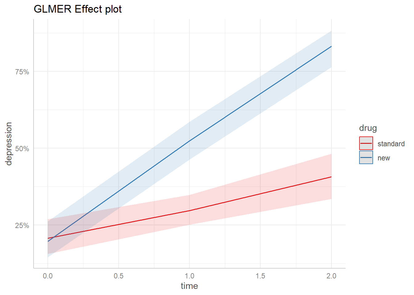
We see the probability of a “Normal” response to the "new" drug increases from less than 25% at time = 0 to over 75% at time = 3. We might consider this plot a population-level estimate since it uses just the fixed effect coefficients.
[2023-02-26 update] To create an effect plot for the GEE model fit by the gee package, we need to call emmeans() directly. When this article was originally published in April 2021, we could use ggeffects as we did above. However, this is no longer the case due to changes in a dependent package. Thanks to Nathaniel Wilson for notifying us of this change.
Below we use the emmeans() function and specify that we want to calculate marginal means for all levels of time and drug, holding diagnose at “severe”. The cov.keep = "time" argument says to keep all levels of time and not average over them. (We need to do this since time is numeric.) The regrid = "response" argument ensures predictions are on the response scale (i.e., probabilities). We pipe the result into as.data.frame(), which returns a data frame suitable for plotting, and save the result as an object called emm_out.
library(emmeans)
emm_out <- emmeans(dep_gee2, specs = c("time", "drug"),
        at = list(diagnose = "severe"),
        cov.keep = "time",
        regrid = "response") %>%
  as.data.frame()
To replicate the ggeffects plot for the glmer() model, we use ggplot2 directly. Notice ggeffects provides the theme_ggeffects() function to assist with this, but we still need to do some extra work to match the color palette ggeffects uses, which is “Set1” from the RColorBrewer package.
library(ggplot2)
ggplot(emm_out) +
  aes(x = time, y = prob, color = drug, fill = drug) +
  geom_line() +
  geom_ribbon(aes(ymin = asymp.LCL, ymax = asymp.UCL,
                  color = NULL), alpha = 0.15) +
  scale_color_brewer(palette = "Set1") +
  scale_fill_brewer(palette = "Set1", guide = NULL) +
  scale_y_continuous(labels = scales::percent) +
  theme_ggeffects() +
  labs(title = "GEE Effect plot", y = "depression")
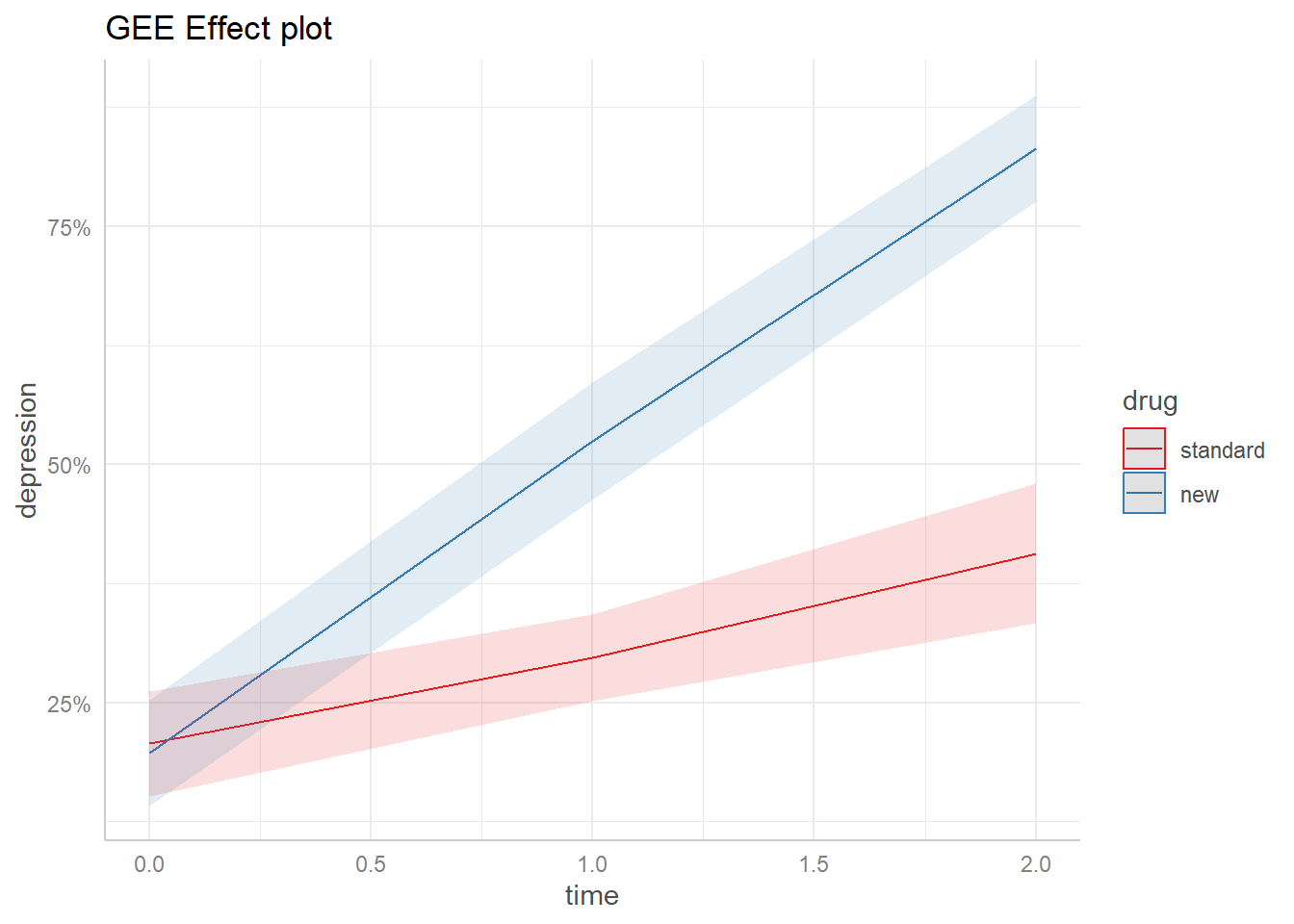
The GEE plot is virtually identical to the glmer plot! For this particular data set, it doesn’t appear to make a difference which model we use.
For an easier process of creating effect plots, you may wish to try the geeglm() function from the geepack package. For example, to replicate the model and effect plot above, we can run the following:
library(geepack) # version 1.3.9
dep_gee4 <- geeglm(depression ~ diagnose + drug*time,
                   data = dat,
                   id = id,
                   family = binomial,
                   corstr = "exchangeable")
# create effect plot
plot(ggemmeans(dep_gee4, terms = c("time", "drug"),
               condition = c(diagnose = "severe"))) +
  ggplot2::ggtitle("GEE Effect plot")
Thanks again to Nathaniel Wilson for this code.
Hopefully you now have a better understanding of how to run and interpret GEE models. There is much more to learn about GEE models, and this article does not pretend to be comprehensive. If you would like to go further, you may wish to explore the geepack R package, which includes a few more GEE functions, a brief vignette, and an introductory article in the Journal of Statistical Software. According to the geepack vignette, “GEEs work best when you have relatively many relatively small clusters in your data.”
R session details
The analysis was done using the R Statistical language (v4.5.2; R Core Team, 2025) on Windows 11 x64, using the packages magrittr (v2.0.4), lme4 (v1.1.37), Matrix (v1.7.4), gee (v4.13.29), emmeans (v2.0.0), ggeffects (v2.3.1) and ggplot2 (v4.0.1).
References
- Agresti, A. (2002). Categorical data analysis (2nd ed.). Wiley.
- Bilder, C., & Loughin, T. (2015). Analysis of categorical data with R. CRC Press.
- Carey, V. (2019). gee: Generalized estimation equation solver (Version 4.13-20). https://CRAN.R-project.org/package=gee
- Harrell, F. (2015). Regression modeling strategies (2nd ed.). Springer.
- Højsgaard, S., Halekoh, U., & Yan, J. (2006) The R package geepack for generalized estimating equations. Journal of Statistical Software, 15(2), 1--11. https://doi.org/10.18637/jss.v015.i02
- Hothorn, T., & Everitt, B. (2014). A handbook of statistical analyses using R (3rd ed.). CRC Press.
- Lenth, R. (2023). emmeans: Estimated marginal means, aka least-squares means (Version 1.8.4-1). https://CRAN.R-project.org/package=emmeans
- Liang, K. Y., & Zeger, S. L. (1986). Longitudinal data analysis using generalized linear models. Biometrika, 73(1) 13--22. https://doi.org/10.1093/biomet/73.1.13
- Lüdecke, D. (2018). ggeffects: Tidy data frames of marginal effects from regression models. Journal of Open Source Software, 3(26), 772. https://doi.org/10.21105/joss.00772.
- R Core Team. (2021). R: A language and environment for statistical computing. R Foundation for Statistical Computing. https://www.R-project.org/
- Wickham, H. (2016). ggplot2: Elegant graphics for data analysis. Springer-Verlag. https://doi.org/10.1007/978-3-319-24277-4
Clay Ford
Statistical Research Consultant
University of Virginia Library
April 22, 2021
Updated February 26, 2023
For questions or clarifications regarding this article, contact statlab@virginia.edu.
View the entire collection of UVA Library StatLab articles, or learn how to cite.