
In R, “growing” an object—extending an atomic vector one element at a time; adding elements one by one to the end of a list; etc.—is an easy way to elicit a mild admonishment from someone reviewing or revising your code. Growing most frequently occurs in the context of for loops: A loop computes a value (or set of values) on each iteration, and it then appends the value(s) to an existing object. The key concern, the issue that actually provokes proscription, is the append step—taking an object of length i and turning it into an object of length i + 1 using c(), append(), or some similar function.
The alternative approach is to preallocate memory in the form of an empty placeholder object with a size as large or larger than that required to contain all the values that the loop will compute. Values of the placeholder object (e.g., NAs) are then filled in—replaced, really—as the loop executes.
The former approach (growing an object) consumes much more memory and generally takes far longer than the latter approach (preallocation). Here, I discuss why this is the case in R, and I compare the speed of several procedures when programmed to grow an object versus when programmed to take advantage of preallocation.
The simple for loop below grows an object by using c() to append the iteration count to an initially empty vector with a length of zero, out. (I include a print step in the body of the loop to show the vector as it exists on each iteration from i = 1 to i = 5.)
out <- c()
for (i in 1:5) {
  out <- c(out, i)
  print(out)
}
[1] 1
[1] 1 2
[1] 1 2 3
[1] 1 2 3 4
[1] 1 2 3 4 5
The trouble is that on each iteration of the loop, the memory currently allocated to hold out isn’t sufficient to hold out plus a new value. R must (1) allocate new memory elsewhere that can stash the now-larger object and then (2) copy values into it. In The R Inferno (2011), a charmingly critical book discussing shortcomings of the R language, Patrick Burns likens this process—occupying increasingly expansive chunks of memory to store a growing object—to suburbanization, and he locates it firmly in the second circle of R hell (just below circle one—the “Floating Point Trap”—and just above circle three—“Failure to Vectorize”).
This phenomenon can be observed directly. The obj_addr() function from the lobstr package returns the memory address of an object. Below, I report the memory address of out on each iteration of the loop:
out <- c()
for (i in 1:5) {
  out <- c(out, i)
  cat('Iteration', i, '| Memory address of `out` is:', lobstr::obj_addr(out), '\n')
}
Iteration 1 | Memory address of `out` is: 0x1155f08e0
Iteration 2 | Memory address of `out` is: 0x1102cb000
Iteration 3 | Memory address of `out` is: 0x1140e6e08
Iteration 4 | Memory address of `out` is: 0x1100a66c8
Iteration 5 | Memory address of `out` is: 0x114476c98
The actual addresses will vary from execution to execution and machine to machine. The point is that the address changes every time out is modified.
Contrast this with a preallocated version of the for loop. I initialize a vector, out, containing five NA values—placeholders that will be overwritten. Printing the memory address of out on each iteration reveals that the memory address remains fixed as I add values to out (or, really, as I perform “in-place modification” of values that were previously NA).
out <- rep(NA, 5)
for (i in 1:5) {
  out[i] <- i
  cat('Iteration', i, '| Memory address of `out` is:', lobstr::obj_addr(out), '\n')
}
Iteration 1 | Memory address of `out` is: 0x124968e68
Iteration 2 | Memory address of `out` is: 0x124968e68
Iteration 3 | Memory address of `out` is: 0x124968e68
Iteration 4 | Memory address of `out` is: 0x124968e68
Iteration 5 | Memory address of `out` is: 0x124968e68
The time cost of the first approach—growing an object—is not insignificant. Below, I use the microbenchmark package to time the two approaches when generating an output vector that simply contains the numbers from 1 to 10,000. The times in milliseconds from 100 tests are shown in the plot that follows.
library(microbenchmark)
library(ggplot2)
n <- 10000
for_loop_timing <- microbenchmark(
  'Grow a vector with c()' = {
    out <- c()
    for (i in 1:n) { out <- c(out, i) }
  },
  'Preallocate memory' = {
    out <- rep(NA, times = n)
    for (i in 1:n) { out[i] <- i }
  },
  times = 100, control = options(warmup = 10)
)
for_medians <- summary(for_loop_timing, unit = 'ms')$median
for_loop_timing$time_ms <- for_loop_timing$time / 1000000
ggplot(for_loop_timing, aes(x = expr, y = time_ms, color = expr)) +
  geom_jitter(width = .1) +
  labs(x = 'Method', y = 'Time (ms)',
       title = 'Time (ms) to generate a vector containing 1, 2, 3, ..., 10000 via a for loop',
       subtitle = '100 times measured for each method',
       caption = 'Horizontal lines are at the median time for each method') +
  ylim(0, max(for_loop_timing$time_ms)*1.5) +
  geom_hline(yintercept = for_medians, color = c('salmon', 'cornflowerblue')) +
  theme(legend.position = 'none') +
  scale_color_manual(values = c('salmon', 'cornflowerblue'))
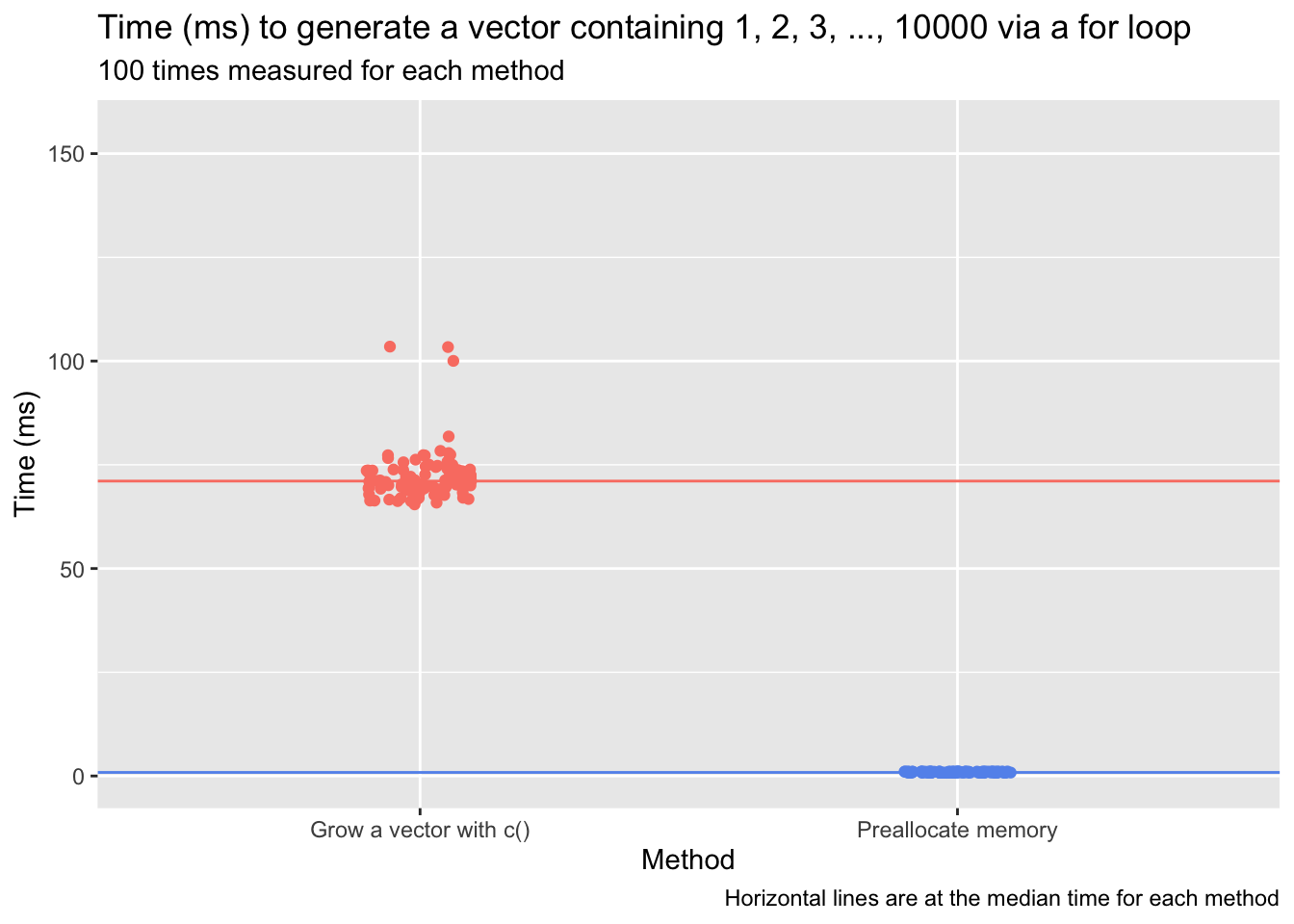
The time required to execute the loop when growing the out vector is dozens of times greater than the time required when preallocating memory (the exact ratio will vary from test to test and machine to machine):
# The summary() method with unit = 'relative' gives the
# relative timings when called on a microbenchmark object:
summary(for_loop_timing, unit = 'relative')[, c('expr', 'min', 'median', 'max', 'neval', 'cld')]
                    expr      min  median      max neval cld
1 Grow a vector with c() 85.19793 82.6825 92.61742   100   b
2     Preallocate memory  1.00000  1.0000  1.00000   100  a
One can similarly compare the total size of the memory allocations that each approach requires. I do so below using the profmem package, which reports the size of memory-allocation events in bytes. The ratio of total memory allocation for the growing approach to total memory allocation for the preallocation approach is ~2,000:1. (This again will vary from run to run and computer to computer.)
library(profmem)
n <- 10000
grow <- profmem({
  out <- c()
  for (i in 1:n) { out <- c(out, i) }
})
preallocate <- profmem({
  out <- rep(NA, times = n)
  for (i in 1:n) { out[i] <- i }
})
cat('Total memory allocation when growing a vector with c() (bytes):', total(grow), '\n')
Total memory allocation when growing a vector with c() (bytes): 200535376
cat('Total memory allocation when preallocating (bytes):', total(preallocate), '\n')
Total memory allocation when preallocating (bytes): 92048
cat('Ratio of total memory allocation, growing a vector vs. preallocating:',
    total(grow) / total(preallocate))
Ratio of total memory allocation, growing a vector vs. preallocating: 2178.596
The example above is quite extreme: An avoidable multi-thousand-fold increase in total memory allocation and a similarly unnecessary eighty-fold increase in run-time are thoroughly off-putting.1 That said, the time and memory costs of growing an object won’t always be so perceptible relative to preallocating, as the increased cost of constantly allocating new memory and moving values to it can be swamped by high costs of operations within the body of a loop. (For example, if I stuck Sys.sleep(60) in the body of the for loops above—forcing R to pause for a minute on every iteration—the added time cost of growing out versus preallocating memory for it would be negligible. Looping from i = 1 to i = 5 would take five minutes—plus or minus some temporal fuzz—no matter what approach I used.) But the relative cost of growing an object can be extreme, and preallocating, when possible, is never going to be a worse option.
This entire topic abuts a conversation about whether to use for loops at all. Some R programmers take a subtle—or sometimes not-so-subtle—pleasure in making known their opposition to loops. This position sometimes emerges from an erroneous view that *apply() functions (apply(), lapply(), etc.) are always faster than explicit for loops. The usual prescription is to take the body of a loop, rewrite it as a function, and pass it to *apply(). Burns takes the legs out from under this position in The R Inferno: “This is not vectorization, it is loop-hiding. The apply function has a for loop in its definition.” (2011, p. 24). (The *apply() functions deserve kudos for preallocating automatically—but their performance does not dominate that of preallocated for loops.)
I’ll happily defend for loops as often-useful (and sometimes necessary) tools. Perhaps I’m writing a process that involves repeatedly sampling from a vector and saving the sampled values, with the sampling probabilities when drawing sample i depending in some way on the value of sample i-1. Being able to reference a previous value via an index (e.g., samples[i-1]) is essential. (Unless, say, I force the value of sample i-1 into the global environment, storing it as an object with a global scope that updates each time a sampling function executes as part of an *apply() function. This is a Faustian bargain all of its own; see the sixth circle of R hell: “Doing Global Assignments” [The R Inferno, 2011, p. 35].)
Preallocation is more complicated when the total number of iterations a loop will complete is indeterminate. A while loop is a natural example: If I randomly sample from the uniform distribution U(0, 10) on each go-around of a loop until I get a (rounded) value greater than or equal to 9.999 (saving all sampled values in a vector), the number of iterations required is unknown in advance. It appears as though one is doomed to grow an object, appending value after value until 9.999 or 10 is sampled. However, a version of preallocation is still on offer: One can preallocate memory in blocks, reserving additional chunks of memory as previously allocated blocks fill up.
Creating an index variable that’s incremented at the end of each iteration of the while loop is one way to accomplish this. One can start by preallocating memory to hold j loop results (e.g., a vector of 1,000 NA values). When the index is a multiple of j, append an additional block of j placeholder values to the end of the existing object. (And if desired, residual placeholder values can be trimmed off at the end.) This does involve some amount of “object growing”—the object has to be copied into a new, expanded memory location every j iterations—but if the while loop executes 4350 times, this approach involves only four such allocations instead of thousands. The time advantage of this approach can be stark: Below, I write two versions of the uniform-distribution sampling process described above (sampling and saving one value from U(0, 10) on each iteration of a while loop until the last-sampled value is at least 9.999). One version grows an output vector, out, on every iteration; the other version allocates memory in the form of 1,000-length blocks of NAs every 1,000 iterations. (I also trim excess NAs at the end of the while loop.) I use the microbenchmark package to compare the time that each version takes to execute, setting the same seed on every test so that the sampling process is identical.
while_loop_timing <- microbenchmark(
  'Grow a vector with c()' = {
    set.seed(999)
    out <- c()
    val <- 0
    while (val < 9.999) {
      val <- round(runif(1, min = 0, max = 10), digits = 3)
      out <- c(out, val)
    }
  },
  'Preallocate memory' = {
    set.seed(999)
    out <- rep(NA, 1000)
    val <- 0
    index <- 1
    while (val < 9.999) {
      val <- round(runif(1, min = 0, max = 10), digits = 3)
      out[index] <- val
      # Check if index is a multiple of 1000; if so, allocate additional memory to hold 1000 more values
      if (index %% 1000 == 0) { out <- c(out, rep(NA, 1000)) }
      index <- index + 1
    }
    out <- out[is.na(out) == F]
  },
  times = 100, control = options(warmup = 10)
)
while_medians <- summary(while_loop_timing, unit = 'ms')$median
while_loop_timing$time_ms <- while_loop_timing$time / 1000000
ggplot(while_loop_timing, aes(x = expr, y = time_ms, color = expr)) +
  geom_jitter(width = .1) +
  labs(x = 'Method', y = 'Time (ms)',
       title = paste0('Time (ms) to draw and save samples from U(0, 10) via a while loop until',
                         '\na rounded value of at least 9.999 is obtained'),
       subtitle = '100 times measured for each method',
       caption = 'Horizontal lines are at the median time for each method') +
  ylim(0, max(while_loop_timing$time_ms)*1.5) +
  geom_hline(yintercept = while_medians, color = c('salmon', 'cornflowerblue')) +
  theme(legend.position = 'none') +
  scale_color_manual(values = c('salmon', 'cornflowerblue'))
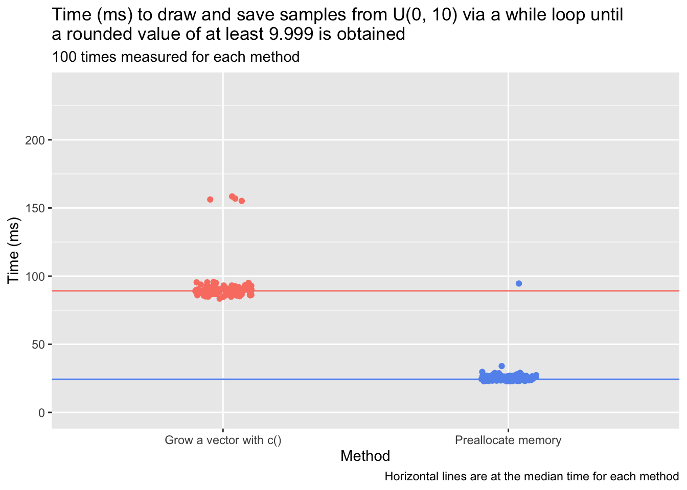
Even with the the occasional costly procedure—copying an object to a new memory address in order to add another 1,000 NA values to it—the process using block preallocation is far faster than the process that grows the output vector with c() on each iteration of the loop.
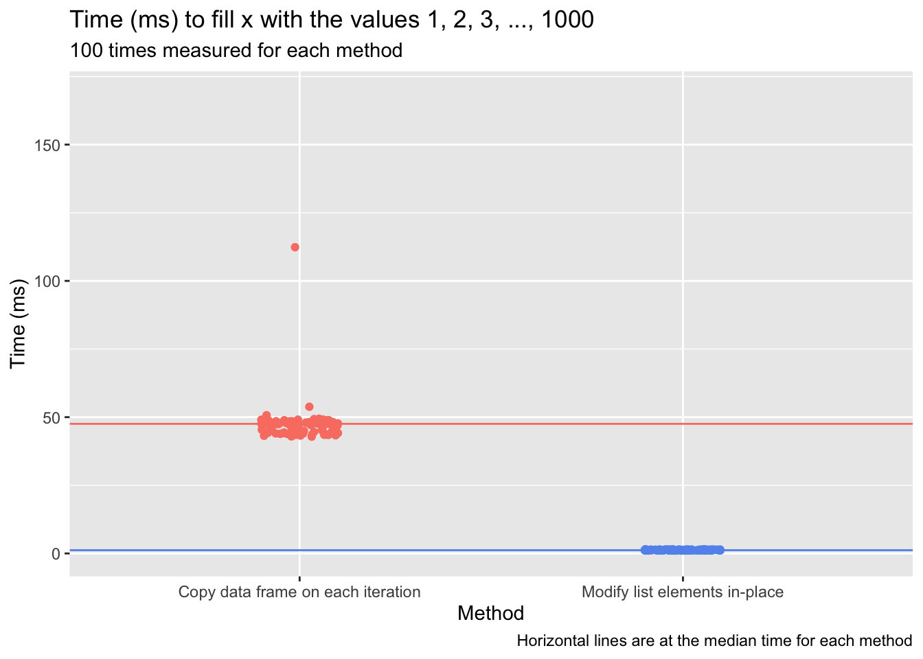
Intuitively, preallocation as exemplified above seems like it would generalize naturally to cases involving data frames: If a 1,000-iteration for loop generates a five-value vector on each go-around that is to be added as a row of a data frame, initialize a 1,000-row/five-column data frame beforehand, and assign each vector of five values to df[i, ] on each iteration from i = 1 to i = 1000. This, however, is not so. R can currently only perform in-place modification (modification without creating a copy of an object, the process that underlies successful preallocation) of certain object classes—atomic vectors, lists, matrices, and arrays being the key ones—that are modified via “primitive” functions written in C. Most R functions and methods, such as those called when modifying a data frame, add a “reference” to an object, and in-place modification is only possible for objects with a single reference (see section 2.5.1 of Wickham’s Advanced R, 2019, for additional details on when and why in-place modification isn’t possible). An occasional workaround to this constraint is to convert a data frame to a list2 and modify its constituent elements, as in the following example:
# The code below appears to involve preallocation (in the form of d),
# but in reality, a copy of d is made on each iteration
d <- data.frame(x = rep(NA, times = 5), y = NA, z = NA)
for (i in 1:5) {
  d[i, 1] <- i
  cat('Iteration', i, '| Memory address of `d` is:', lobstr::obj_addr(d), '\n')
}
Iteration 1 | Memory address of `d` is: 0x121bb6e68
Iteration 2 | Memory address of `d` is: 0x121bb70e8
Iteration 3 | Memory address of `d` is: 0x121bb72c8
Iteration 4 | Memory address of `d` is: 0x121bb74f8
Iteration 5 | Memory address of `d` is: 0x121bb7728
# The alternative approach, which successfully implements preallocation,
# is to convert d to a list and then modify values in-place
d <- data.frame(x = rep(NA, times = 5), y = NA, z = NA)
d_list <- as.list(d)
for (i in 1:5) {
  d_list[[1]][i] <- i
  cat('Iteration', i, '| Memory address of `d_list` is:', lobstr::obj_addr(d_list), '\n')
}
Iteration 1 | Memory address of `d_list` is: 0x125b47258
Iteration 2 | Memory address of `d_list` is: 0x125b47258
Iteration 3 | Memory address of `d_list` is: 0x125b47258
Iteration 4 | Memory address of `d_list` is: 0x125b47258
Iteration 5 | Memory address of `d_list` is: 0x125b47258
The speed differential of these approaches is notable. I time each below using microbenchmark, with the loops now extended to involve 1,000 value-insertions instead of five.
df_list_timing <- microbenchmark(
  'Copy data frame on each iteration' = {
    d <- data.frame(x = rep(NA, times = 5), y = NA, z = NA)
    for (i in 1:1000) { d[i, 1] <- i }
  },
  'Modify list elements in-place' = {
    d <- data.frame(x = rep(NA, 1000), y = NA, z = NA)
    d_list <- as.list(d)
    for (i in 1:1000) { d_list[[1]][i] <- i }
  },
  times = 100, control = options(warmup = 10)
)
df_list_medians <- summary(df_list_timing, unit = 'ms')$median
df_list_timing$time_ms <- df_list_timing$time / 1000000
ggplot(df_list_timing, aes(x = expr, y = time_ms, color = expr)) +
  geom_jitter(width = .1) +
  labs(x = 'Method', y = 'Time (ms)',
       title = paste0('Time (ms) to fill x with the values 1, 2, 3, ..., 1000'),
       subtitle = '100 times measured for each method',
       caption = 'Horizontal lines are at the median time for each method') +
  ylim(0, max(df_list_timing$time_ms)*1.5) +
  geom_hline(yintercept = df_list_medians, color = c('salmon', 'cornflowerblue')) +
  theme(legend.position = 'none') +
  scale_color_manual(values = c('salmon', 'cornflowerblue'))
Preallocation is viable in R when adding values to atomic vectors, lists, matrices, and arrays.3 The complication exemplified above—that modifying a data frame using standard subsetting and indexing tools creates a copy of the data frame—is an unfortunate constraint. Note too that preallocation is hardly the sole way to speed up iterative processes in R. Parallelization, for example, distributes work across multiple computer cores, which can slice down run-times significantly. And if every nanosecond counts, turning to a faster language—a compiled language, usually—like Go or C for a process rewrite may be an attractive option. But when R code involves a loop, with output being saved to an atomic vector, list, matrix, or array, the prescription is an easy one to provide: Preallocate.
R session details
The analysis was done using the R Statistical language (v4.5.2; R Core Team, 2025) on Windows 11 x64, using the packages profmem (v0.7.0), microbenchmark (v1.5.0) and ggplot2 (v4.0.1).
References
- Burns, P. (2011). The R inferno. https://www.burns-stat.com/pages/Tutor/R_inferno.pdf
- Wickham, H. (2019). Advanced R (2nd ed.). CRC Press. https://adv-r.hadley.nz
Jacob Goldstein-Greenwood
Research Data Scientist
University of Virginia Library
September 22, 2023
I have stacked the deck somewhat by growing vectors with
c()in the examples above. An alternative approach that still grows a vector is to initialize an empty, zero-length vector and then to add a new value to it viavec[i] <- valon each iteration of a loop. This approach, while still slower than preallocating memory, is markedly faster than growing a vector withc():↩︎n <- 10000 times <- microbenchmark( 'Grow a vector via out[i]' = { out <- c() for (i in 1:n) { out[i] <- i } }, 'Preallocate memory' = { out <- rep(NA, times = n) for (i in 1:n) { out[i] <- i } }, times = 100, control = options(warmup = 10) ) # Relative speed (ratios): summary(times, unit = 'relative')[, c('expr', 'min', 'median', 'max', 'neval', 'cld')]expr min median max neval cld 1 Grow a vector via out[i] 2.058336 2.062458 0.9352426 100 b 2 Preallocate memory 1.000000 1.000000 1.0000000 100 a- The immediate rejoinder may be: “A data frame is a list!” Although
is.list(data.frame(x = 1, y = 1))indeed returnsTRUEwithout hesitation, a data frame is a unique class of object, with its own associated methods for accomplishing tasks like subsetting and value modification. Consider the difference between[and[.data.frame: The former is a primitive C function; the latter is a method for data frames that involves the execution of a slue of R code.c(1, 2, 3)[1]invokes the former;data.frame(x = 1, y = 1)[1, ]invokes the latter.[.data.framecreates an additional reference to the data frame the method is applied to—rendering in-place modification impossible.↩︎ The viability of preallocation when working with those data structures can be checked directly:↩︎
# Preallocate atomic vector
vec <- rep(NA, 2)
for (i in 1:2) {
  vec[i] <- i
  cat(lobstr::obj_addr(vec), '... ')
}
0x153a543c8 ... 0x153a543c8 ...# Preallocate matrix mat <- matrix(rep(NA, 4), nrow = 2) for (i in 1:2) { mat[i, 1] <- i cat(lobstr::obj_addr(mat), '... ') }0x1272c3a88 ... 0x1272c3a88 ...# Preallocate array arr <- array(rep(NA, 8), dim = c(2, 2, 2)) for (i in 1:2) { arr[1, 1, i] <- i cat(lobstr::obj_addr(arr), '... ') }0x121d5e7c8 ... 0x121d5e7c8 ...# Preallocate list ll <- list(NA, NA) for (i in 1:2) { ll[i] <- i cat(lobstr::obj_addr(ll), '... ') }0x127206348 ... 0x127206348 ...
For questions or clarifications regarding this article, contact statlab@virginia.edu.
View the entire collection of UVA Library StatLab articles, or learn how to cite.