
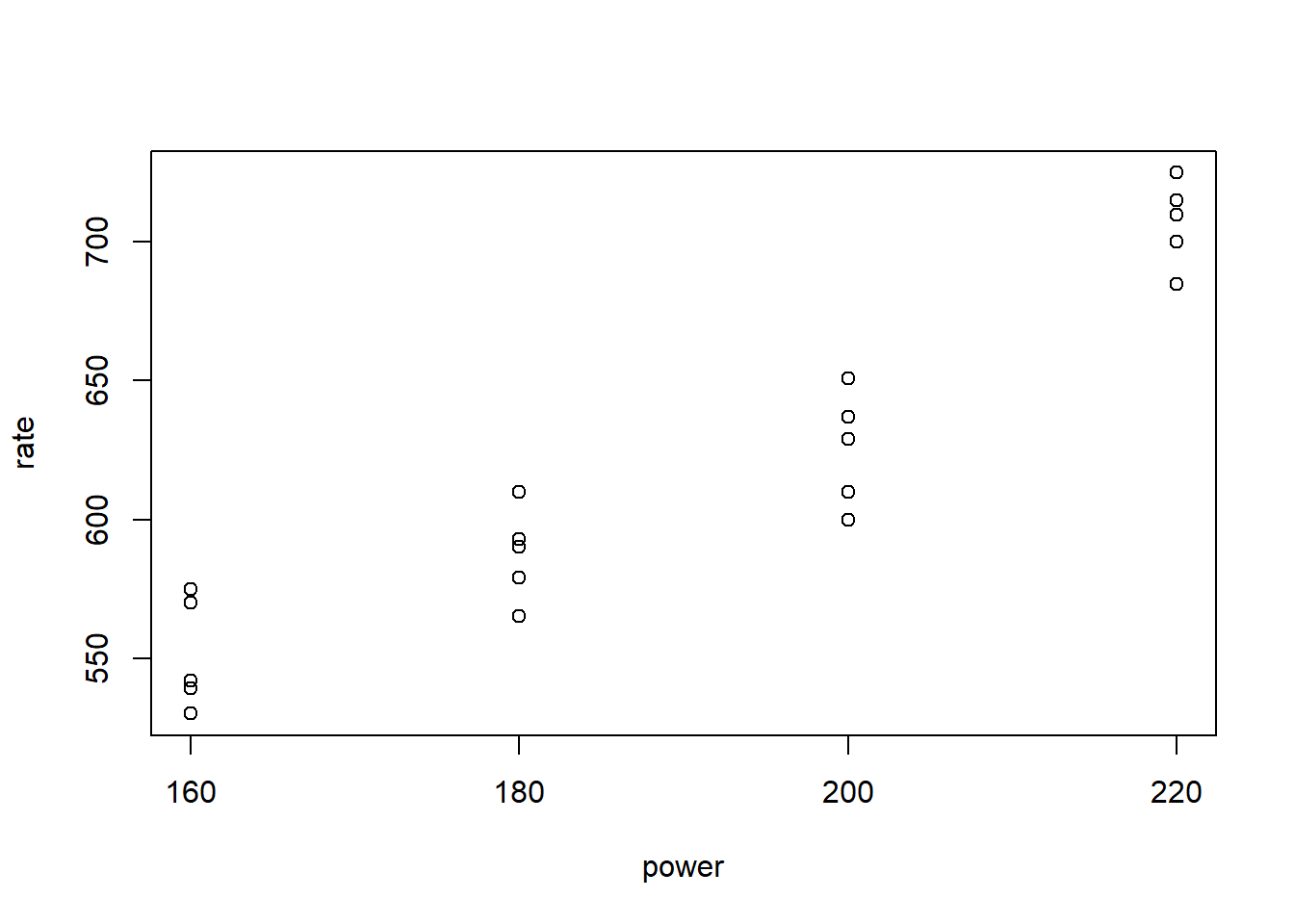
Consider the following data from the text Design and Analysis of Experiments, 7th ed. (Montgomery, 2009, Table 3.1). It has two variables: power and rate. power is a discrete setting on a tool used to etch circuits into a silicon wafer. There are four levels to choose from. rate is the distance etched measured in Angstroms per minute. (An Angstrom is one ten-billionth of a meter.) Of interest is how (or if) the power setting affects the etch rate. Below we enter the small data set by hand into R and create a quick plot. The plot suggests higher power settings lead to higher etch rates.
# Table 3.1
power <- rep(c(160, 180, 200, 220), 5)
rate <- c(575, 565, 600, 725,
          542, 593, 651, 700,
          530, 590, 610, 715,
          539, 579, 637, 685,
          570, 610, 629, 710)
etch <- data.frame(rate, power)
stripchart(rate ~ power, data = etch, pch = 1,
           vertical = TRUE, xlab = "power")
A formal statistical analysis of this data requires a linear model. To perform the analysis in R, we need to define the power variable as a factor. This tells R that power is a categorical variable and to treat it as such in a modeling procedure. But in addition, we may want to further specify that the levels of power are ordered. Power level 160 is less than 180, and 180 is less than 200, and so on. This is additional information we may want to account for. We can define power as an ordered factor in R using the ordered() function. We do that below and save the ordered factor version as powerF. Notice that calling head() to view the first 6 values of powerF shows us the ordering of the levels: 160 < 180 < 200 < 220.
etch$powerF <- ordered(etch$power)
head(etch$powerF)
  [1] 160 180 200 220 160 180
  Levels: 160 < 180 < 200 < 220
It’s important to note that R is storing powerF internally as integers, which we can see by calling unclass() or as.integer() on the variable. (We'll make use of this fact in the next plot we create.)
unclass(etch$powerF)
[1] 1 2 3 4 1 2 3 4 1 2 3 4 1 2 3 4 1 2 3 4
attr(etch$powerF,"levels")
[1] "160" "180" "200" "220"
Now let’s formally analyze the data using the lm() function in R. This is equivalent to performing a one-way ANOVA. Below we model rate as a function of the ordered factor powerF and pipe the result into the summary() function using base R’s native forward pipe operator, |>, introduced in version 4.1.0.
lm(rate ~ powerF, data = etch) |> summary()
  Call:
  lm(formula = rate ~ powerF, data = etch)

  Residuals:
     Min     1Q Median     3Q    Max
   -25.4  -13.0    2.8   13.2   25.6

  Coefficients:
              Estimate Std. Error t value Pr(>|t|)
  (Intercept)  617.750      4.085 151.234  < 2e-16 ***
  powerF.L     113.011      8.169  13.833 2.56e-10 ***
  powerF.Q      22.700      8.169   2.779   0.0134 *
  powerF.C       9.347      8.169   1.144   0.2694
  ---
  Signif. codes:  0 '***' 0.001 '**' 0.01 '*' 0.05 '.' 0.1 ' ' 1

  Residual standard error: 18.27 on 16 degrees of freedom
  Multiple R-squared:  0.9261, Adjusted R-squared:  0.9122
  F-statistic:  66.8 on 3 and 16 DF,  p-value: 2.883e-09
At the bottom of the output is the familiar ANOVA test result. The F-statistic is large and the p-value is tiny, which provides evidence that the mean rates between the four power levels are different. (We have statistically sanctified what we saw in the plot.) In addition, the adjusted R-squared suggests power explains about 91% of the variability we’re seeing in the etch rates. But what about the rest? What are these mysterious “powerF.L”, “powerF.Q”, and “powerF.C” labels? What do their estimates mean? What are the hypothesis tests associated with them?
The quick answers to these questions are that the L, Q, and C stand for linear, quadratic, and cubic; that the coefficients don't have a ready interpretation; and that each hypothesis is a test for trend.
The “powerF.L” entry is a test for linear trend. The null is no linear trend (i.e., a flat line). The large t-value provides evidence against this. Again, this is not a surprise. Looking at the plot above, we can visualize a straight line over the points.
The “powerF.Q” entry is a test for quadratic trend. The null is no quadratic trend (i.e., a straight line). The t-value of 2.8 provides some evidence against this. This is less obvious in the plot, though we can perhaps imagine a slight curve superimposed over the data.
The “powerF.C” entry is a test for cubic trend. The null is no cubic trend (i.e., a straight or quadratic line). The t-value of 1.1 is small, and the p-value is quite large. There doesn’t appear to be any cubic trend in the data.
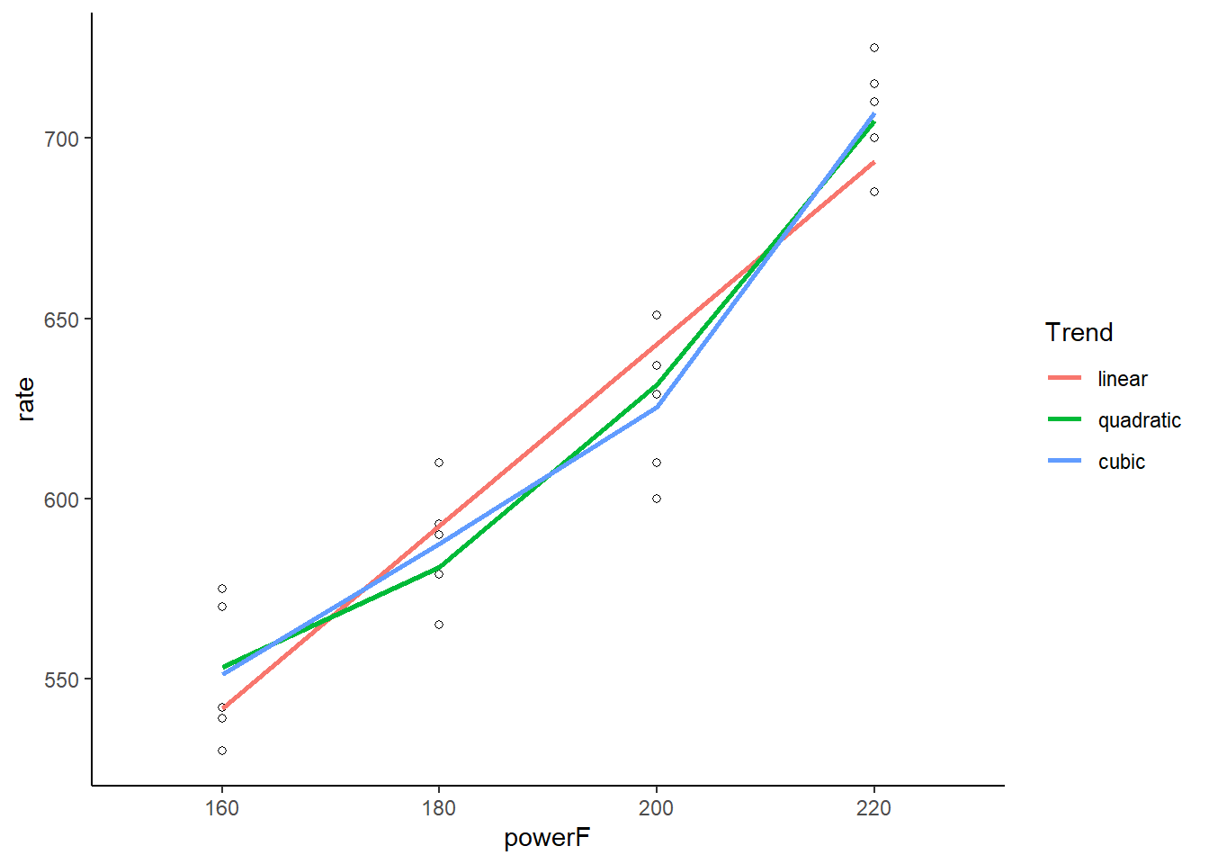
We can visualize these trends using ggplot(). Below we call geom_smooth() three times to plot linear, quadratic and cubic lines using lm(). Notice we have to unclass() the powerF variable to make this work. Defining the colors as “1”, “2”, and “3” is an easy way to force ggplot() to create a legend and place the labels in that order. We notice there isn’t much difference between the fitted quadratic and cubic lines, visually demonstrating why the cubic trend test was not “significant.”
library(ggplot2)
ggplot(etch) +
  aes(x = powerF, y = rate) +
  geom_point(shape = 1) +
  geom_smooth(aes(x = unclass(powerF), color = "1"),
              formula = y ~ x,
              method = lm, se = FALSE) +
  geom_smooth(aes(x = unclass(powerF), color = "2"),
              formula = y ~ poly(x, 2),
              method = lm, se = FALSE) +
  geom_smooth(aes(x = unclass(powerF), color = "3"),
              formula = y ~ poly(x, 3),
              method = lm, se = FALSE) +
  scale_color_discrete("Trend", labels = c("linear", "quadratic", "cubic")) +
  theme_classic()
If you’re thinking these tests for trend look a lot like a polynomial model, you’re right. That’s basically what it is. In fact, we get identical test results (i.e., the same test statistics and p-values) if we simply fit a 3-degree polynomial model to the original numeric power variable.
lm(rate ~ poly(power, 3), data = etch) |> summary()
  Call:
  lm(formula = rate ~ poly(power, 3), data = etch)

  Residuals:
     Min     1Q Median     3Q    Max
   -25.4  -13.0    2.8   13.2   25.6

  Coefficients:
                  Estimate Std. Error t value Pr(>|t|)
  (Intercept)      617.750      4.085 151.234  < 2e-16 ***
  poly(power, 3)1  252.700     18.267  13.833 2.56e-10 ***
  poly(power, 3)2   50.759     18.267   2.779   0.0134 *
  poly(power, 3)3   20.900     18.267   1.144   0.2694
  ---
  Signif. codes:  0 '***' 0.001 '**' 0.01 '*' 0.05 '.' 0.1 ' ' 1

  Residual standard error: 18.27 on 16 degrees of freedom
  Multiple R-squared:  0.9261, Adjusted R-squared:  0.9122
  F-statistic:  66.8 on 3 and 16 DF,  p-value: 2.883e-09
We also get the same test results if we unclass() the ordered factor version of power and fit a 3-degree polynomial model.
lm(rate ~ poly(unclass(powerF), 3), data = etch) |> summary()
  Call:
  lm(formula = rate ~ poly(unclass(powerF), 3), data = etch)

  Residuals:
     Min     1Q Median     3Q    Max
   -25.4  -13.0    2.8   13.2   25.6

  Coefficients:
                            Estimate Std. Error t value Pr(>|t|)
  (Intercept)                617.750      4.085 151.234  < 2e-16 ***
  poly(unclass(powerF), 3)1  252.700     18.267  13.833 2.56e-10 ***
  poly(unclass(powerF), 3)2   50.759     18.267   2.779   0.0134 *
  poly(unclass(powerF), 3)3   20.900     18.267   1.144   0.2694
  ---
  Signif. codes:  0 '***' 0.001 '**' 0.01 '*' 0.05 '.' 0.1 ' ' 1

  Residual standard error: 18.27 on 16 degrees of freedom
  Multiple R-squared:  0.9261, Adjusted R-squared:  0.9122
  F-statistic:  66.8 on 3 and 16 DF,  p-value: 2.883e-09
Did you notice the coefficients and standard errors of these two models differ from the first model with the ordered factor? That’s because the ordered factor model uses a contrast. A contrast is a matrix that transforms a series of 0/1 dummy variables into columns that can be estimated in a modeling routine. The default contrast for ordered factors in R is the polynomial contrast. We can see the contrast R uses by calling the contr.poly() function. Simply tell it how many levels your categorical variable has. In our case we have 4.
contr.poly(4)
               .L   .Q         .C
  [1,] -0.6708204  0.5 -0.2236068
  [2,] -0.2236068 -0.5  0.6708204
  [3,]  0.2236068 -0.5 -0.6708204
  [4,]  0.6708204  0.5  0.2236068
That’s the contrast used to convert dummy variables of an ordered factor into a model matrix. Let’s demonstrate. Below we generate a 4-column matrix of dummy variables for the power variable. There is one row per observation and one column per level of power. A 1 in a row identifies membership in one of the four power categories.
Xpower <- sapply(c(160, 180, 200, 220),
               function(x)ifelse(etch$power==x, 1, 0))
colnames(Xpower) <- c("160", "180", "200", "220")
head(Xpower)
       160 180 200 220
  [1,]   1   0   0   0
  [2,]   0   1   0   0
  [3,]   0   0   1   0
  [4,]   0   0   0   1
  [5,]   1   0   0   0
  [6,]   0   1   0   0
Now we multiply the dummy variable matrix by the polynomial contrast to obtain a model matrix that is estimable.
Xpower %*% contr.poly(4)
                .L   .Q         .C
   [1,] -0.6708204  0.5 -0.2236068
   [2,] -0.2236068 -0.5  0.6708204
   [3,]  0.2236068 -0.5 -0.6708204
   [4,]  0.6708204  0.5  0.2236068
   [5,] -0.6708204  0.5 -0.2236068
   [6,] -0.2236068 -0.5  0.6708204
   [7,]  0.2236068 -0.5 -0.6708204
   [8,]  0.6708204  0.5  0.2236068
   [9,] -0.6708204  0.5 -0.2236068
  [10,] -0.2236068 -0.5  0.6708204
  [11,]  0.2236068 -0.5 -0.6708204
  [12,]  0.6708204  0.5  0.2236068
  [13,] -0.6708204  0.5 -0.2236068
  [14,] -0.2236068 -0.5  0.6708204
  [15,]  0.2236068 -0.5 -0.6708204
  [16,]  0.6708204  0.5  0.2236068
  [17,] -0.6708204  0.5 -0.2236068
  [18,] -0.2236068 -0.5  0.6708204
  [19,]  0.2236068 -0.5 -0.6708204
  [20,]  0.6708204  0.5  0.2236068
Notice this is the same model.matrix() that is used when we model the ordered factor with lm(). (The column of ones is for the intercept.)
lm(rate ~ powerF, data = etch) |> model.matrix()
     (Intercept)   powerF.L powerF.Q   powerF.C
  1            1 -0.6708204      0.5 -0.2236068
  2            1 -0.2236068     -0.5  0.6708204
  3            1  0.2236068     -0.5 -0.6708204
  4            1  0.6708204      0.5  0.2236068
  5            1 -0.6708204      0.5 -0.2236068
  6            1 -0.2236068     -0.5  0.6708204
  7            1  0.2236068     -0.5 -0.6708204
  8            1  0.6708204      0.5  0.2236068
  9            1 -0.6708204      0.5 -0.2236068
  10           1 -0.2236068     -0.5  0.6708204
  11           1  0.2236068     -0.5 -0.6708204
  12           1  0.6708204      0.5  0.2236068
  13           1 -0.6708204      0.5 -0.2236068
  14           1 -0.2236068     -0.5  0.6708204
  15           1  0.2236068     -0.5 -0.6708204
  16           1  0.6708204      0.5  0.2236068
  17           1 -0.6708204      0.5 -0.2236068
  18           1 -0.2236068     -0.5  0.6708204
  19           1  0.2236068     -0.5 -0.6708204
  20           1  0.6708204      0.5  0.2236068
  attr(,"assign")
  [1] 0 1 1 1
  attr(,"contrasts")
  attr(,"contrasts")$powerF
  [1] "contr.poly"
The latter two models that explicitly modeled a 3-degree polynomial did not use a contrast. Instead, the actual power values were squared and cubed.
Is there an advantage to using one over the other? Maybe we should have just used polynomial regression instead of creating an ordered factor. Fox and Weisberg (2019) tell us contr.poly() is appropriate when the levels of your ordered factor are equally spaced and balanced. That is the case for the power variable. Each level of power is separated by 20 units, and we have five observations for each level. If we have an ordered factor that does not have equal spacing and/or is not balanced, we’re better off performing polynomial regression via the poly() function.
It’s worth noting that even though we have power saved as an ordered factor and modeled with a polynomial contrast, we can still perform follow-up analyses usually associated with standard unordered categorical variables. For example, using the emmeans package we can make pairwise comparisons.
library(emmeans)
lm(rate ~ powerF, data = etch) |>
  emmeans(specs = "powerF") |>
  pairs()
   contrast  estimate   SE df t.ratio p.value
   160 - 180    -36.2 11.6 16  -3.133 0.0294
   160 - 200    -74.2 11.6 16  -6.422 <.0001
   160 - 220   -155.8 11.6 16 -13.485 <.0001
   180 - 200    -38.0 11.6 16  -3.289 0.0216
   180 - 220   -119.6 11.6 16 -10.352 <.0001
   200 - 220    -81.6 11.6 16  -7.063 <.0001

  P value adjustment: tukey method for comparing a family of 4 estimates
Hopefully you now have a better understanding of what’s happening in R when you set a factor as ordered and use it in a linear model.
R session details
The analysis was done using the R Statistical language (v4.5.1; R Core Team, 2025) on Windows 11 x64, using the packages emmeans (v1.11.2.8) and ggplot2 (v3.5.2).
References
- Fox, J., & Weisberg, S. (2019). An R companion to applied regression (3rd ed.). Sage. https://socialsciences.mcmaster.ca/jfox/Books/Companion/
- Lenth, R. (2023). emmeans: Estimated marginal means, aka least-squares means (Version 1.8.5). https://cran.r-project.org/package=emmeans
- Montgomery, D. (2009). Design and analysis of experiments (7th ed.). Wiley.
- R Core Team. (2023). R: A language and environment for statistical computing. R Foundation for Statistical Computing. https://www.R-project.org
Clay Ford
Statistical Research Consultant
University of Virginia Library
July 1, 2021
For questions or clarifications regarding this article, contact statlab@virginia.edu.
View the entire collection of UVA Library StatLab articles, or learn how to cite.