Theil-Sen Regression: Programming and Understanding an Outlier-Resistant Alternative to Least Squares

Least squares is so frequently the method by which linear regressions are estimated that in many write-ups of analyses, explicit mention of the method is omitted. Authors save the ink or pixels otherwise consumed by “least squares” and let it simply be inferred. This is an understandable elision: You could make good money repeatedly betting that when someone says that they fit a linear regression, they did so via least squares. But alternative estimation methods are on offer—and are sometimes preferable. In the face of outliers and odd data points, a regression coefficient estimated via least squares is touchy. An estimate of the relationship between x and y can be rendered woefully inaccurate by a relatively small number of extreme observations. (This matter, and a method of diagnosis, has been considered elsewhere in these digital pages.) Other methods of estimation can greatly mitigate that threat.

One alternative to least-squares regression when estimating a linear relationship between x and y is Theil-Sen regression. In simple linear regression fit by least squares, the coefficient of predictor x (the slope between x and y) and the intercept are chosen such that the value of \(\sum_{i=1}^{n} (y_i - \hat{y}_i)^2\) (the sum of squared residuals) is minimized. In Theil-Sen regression, the slope is calculated by taking the median of the slopes between each pair of points in the data. (For a pair of points, \((x_i, y_i)\) and \((x_j, y_j)\), the slope is calculated as \((y_j - y_i) / (x_j - x_i)\).) An intercept can be calculated to accompany the Theil-Sen slope estimate as well: For each point, \((x_i, y_i)\), solve \(y_i = mx_i + b_i\) for \(b_i\), where m is the Theil-Sen slope (i.e., find the intercept of the line with the calculated Theil-Sen slope that passes through each point); then take the median of those intercepts (Young, p. 201).

The method was described by Theil in 1950, and Sen developed it in 1968 to address cases in which pairs of points share the same x values, which would mean dividing by zero in the slope calculation and thus make the slope indefinite. His solution was simply to omit indefinite slopes; that is, to only calculate \((y_j - y_i)/(x_j - x_i)\) if \(x_i \ne x_j\).

The accuracy of Theil-Sen estimation can far outstrip that of least squares in the presence of outliers and odd data points. (It is one of several methods collectively falling under the heading of “robust regression”—methods that are more resistant than least squares to outliers and violations of least-squares regression assumptions like error normality and error-variance homogeneity.) To catch the intuition as to why Theil-Sen estimation can produce accurate slope estimates in the face of arbitrarily extreme observations, consider the relative resistance of the median versus the mean to outliers in a given set of values: The mean and median of the set \(\{1, 2, 3, 4, 5\}\) are both 3; however, if the largest number in the set is replaced with 5000, the mean skyrockets to 1002, whereas the median stays exactly where it was at a cool, unruffled value of 3. This comparison between means and medians can be generalized to the context of regression: The least-squares estimate of simple regression slope can be conceptualized as a weighted average of pairwise slopes (with weights given by \((x_j - x_i)^2\); see Wilcox, p. 29). Extreme points yank that calculation around in the same way that swapping out 5 for 5000 in the example above inflates the mean. The median of slopes, however, can survive extreme values without being dynamited (or miniaturized, as the case may be) in the same way.

Below, I develop a simulation to demonstrate the stark difference in accuracy between Theil-Sen and least-squares estimation when estimating bivariate linear relationships in data sets containing observations that have been arbitrarily inflated or deflated and yanked left or right. To make a comparative simulation possible, I need a function for calculating a Theil-Sen slope given a set of x and y values. Several R packages on CRAN contain such functions, but it’s reasonably straightforward to write one’s own—and programming an estimator is useful for understanding how it works. (See the appendix at the bottom of this article for a partial list of CRAN packages containing Theil-Sen estimators, as well as a discussion of an inaccuracy that one of the packages—mblm—has when estimating Theil-Sen regressions on data containing NA values.)

The function takes a two-column matrix or data frame as an input, and it treats the first column as the predictor (x) and the second column as the outcome (y; this can be reversed by setting the x_is_first_col argument to FALSE). The series of if expressions that begin the function validate and modify the input as needed. Observations with an NA value in either column are removed from the data (and an alert is printed). The function then determines the maximum possible number of point-to-point slopes that can be calculated from the n complete observations, \(n(n-1)/2\), after which it calculates the slope between each pair of points that don’t share an x value and takes the median of those values: This is the Theil-Sen estimate of the relationship. The Theil-Sen intercept is then calculated by taking the median of the intercepts of the lines with the Theil-Sen slope passing through each observation.

theil_sen <- function(mat, x_is_first_col = TRUE) {
  # Validate input
  if (inherits(mat, c('matrix', 'data.frame')) == FALSE) {
    stop('mat must be a matrix or data frame', call. = FALSE)
  }
  if (ncol(mat) != 2) {
    stop('mat must have exactly two columns', call. = FALSE)
  }
  if (FALSE %in% sapply(mat, is.numeric)) {
    stop('The columns of mat must be numeric', call. =)
  }
  if (x_is_first_col == FALSE) {
    mat <- mat[, 2:1]
    message('x_first_col is FALSE: First and second columns of input data have been reversed')
  }
  if (length(unique(mat[, 1])) == 1) {
    stop("All x values are identical; Theil-Sen estimator can't be calculated", call. = FALSE)
  }
  if (TRUE %in% is.na(mat)) {
    orig_nrow <- nrow(mat); mat <- mat[complete.cases(mat), ]; post_nrow <- nrow(mat)
    n_removed <- orig_nrow - post_nrow
    message(n_removed, ' row', ifelse(n_removed > 1, 's', ''), ' containing NA removed')
  }
  # Set up process
  x <- mat[, 1]
  y <- mat[, 2]
  n <- length(x)
  max_n_slopes <- (n * (n - 1)) / 2
  slopes <- vector(mode = 'list', length = max_n_slopes) # list of NULL elements
  add_at <- 1
  # Calculate point-to-point slopes if x_i != x_j
  for (i in 1:(n - 1)) {
    slopes_i <- lapply((i + 1):n, function(j) if (x[j] != x[i]) { (y[j] - y[i]) / (x[j] - x[i]) })
    slopes[add_at:(add_at + length(slopes_i) - 1)] <- slopes_i
    add_at <- add_at + length(slopes_i)
  }
  # Calculate Theil-Sen slope
  slopes <- unlist(slopes) # drop NULL elements (indefinite slopes/unfilled list entries)
  theil_sen_slope <- median(slopes, na.rm = TRUE)
  # Calculate Theil-Sen intercept
  intercepts <- y - (theil_sen_slope * x)
  theil_sen_intercept <- median(intercepts, na.rm = TRUE)
  # Return
  c('Theil-Sen intercept' = theil_sen_intercept, 'Theil-Sen slope' = theil_sen_slope)
}

Using this function, I compare the accuracy of Theil-Sen and least-squares regression slopes in data sets with increasing proportions of corrupted points. For a given data set, I simulate 100 x values by randomly sampling from \(N(0, 16)\). I then generate a y value for each x value via the equation \(y = 2x + \epsilon,~\epsilon\sim N(0, 4)\). With x and y values in hand, I select a given proportion of observations to corrupt, picking points at random. For each of the selected points, I randomly select a value from a uniform distribution ranging from 2.0 to 4.0, and I randomly select either 1.0 or -1.0; I then multiply the point’s y value by those two values. I repeat this process for the x value of each point. (I.e., increasing or decreasing each corrupted observation’s x and y values by factors of 2.0 to 4.0. I refer to these observations as “corrupted points” instead of “outliers,” as this process can result in some observations being shifted such that they still fall within the general trend of the x/y relationship.) I repeat this data-simulation process 500 times for each proportion of corrupted points, \(\{0, 0.05, 0.10, ..., 0.40\}\), and I calculate the Theil-Sen and least-squares regression slope estimates in each data set. The true (population-level) slope in each data set (to which the Theil-Sen and least-squares slopes can be compared) is 2.0. The simulation results are shown in the plot below.

# Set up simulation
library(ggplot2)
set.seed(99)
b <- 500
outlier_proportions <- seq(0, .40, by = .05)
out <- data.frame('ts_slope' = NA,
                  'lm_slope' = NA,
                  'prop' = as.character(rep(outlier_proportions, each = b)))

# Function to generate and corrupt x and y values
sample_and_corrupt <- function(n, x_sd, b0, b1, e_sd, prop, multiplier_min, multiplier_max) {
    x <- rnorm(n, 0, x_sd)
    y <- b0 + b1*x + rnorm(n, 0, e_sd)
    corrupt <- sample(length(y), size = length(y)*prop, replace = FALSE)
    y[corrupt] <- y[corrupt]*runif(length(corrupt), multiplier_min, multiplier_max)*
      sample(c(-1, 1), length(corrupt), replace = TRUE)
    x[corrupt] <- x[corrupt]*runif(length(corrupt), multiplier_min, multiplier_max)*
      sample(c(-1, 1), length(corrupt), replace = TRUE)
    matrix(c(x, y), byrow = FALSE, ncol = 2)
}

# Run simulation
for (i in 1:length(outlier_proportions)) {
  res <- replicate(b, {
    dat <- sample_and_corrupt(n = 100, x_sd = 4, b0 = 0, b1 = 2, e_sd = 2,
                              prop = outlier_proportions[i], multiplier_min = 2, multiplier_max = 4)
    c(theil_sen(dat)[2], coef(lm(dat[, 2] ~ dat[, 1]))[2])
  }, simplify = FALSE)
  res <- do.call(rbind, res)
  out[(b*(i-1) + 1):(b*i), c('ts_slope', 'lm_slope')] <- res
}

# Reshape output for plotting
out_long <- tidyr::pivot_longer(out, -'prop', names_to = 'estimator', values_to = 'beta')

# Calculate median estimate at each proportion for each estimator
medians <- aggregate(out_long$beta, by = list(out_long$prop, out_long$estimator), median)
colnames(medians) <- c('prop', 'estimator', 'val')

# Labels for plotting
title_lab <- paste0('Theil-Sen and least-squares coefficients for samples',
                    ' with varying proportions of corrupted observations')
subtitle_lab <- expression(paste('Data-generating process (pre-corruption): ',
                                 y == 2.0*x + epsilon, ', ', x %~% N(0, 16), ', ', epsilon %~% N(0, 4)))
caption_lab <- paste0('Each sample contains 100 observations',
                      '\nObservations corrupted by increasing or decreasing the x and y values of',
                      ' selected points by randomly selected factors between 2.0 and 4.0',
                      '\nLines reflect medians, and point clouds are dodged to the left and right',
                      ' of a given x-axis value solely for visibility')

# Plot
ggplot(out_long) +
  geom_jitter(aes(prop, beta, color = estimator), position = position_dodge2(.6), size = .5) +
  geom_point(data = medians, aes(prop, val, group = estimator), position = position_dodge2(.6)) +
  geom_line(data = medians, aes(prop, val, group = estimator), position = position_dodge2(.6)) +
  geom_hline(aes(yintercept = 2)) +
  labs(title = title_lab, subtitle = subtitle_lab, caption = caption_lab,
       x = 'Proportion of corrupted observations', y = 'Estimated slope',
       color = 'Estimator', linetype = 'Estimator') +
  scale_color_manual(values = c('#8e7dbe', '#99c1b9'),
                     labels = c('Least-squares regression', 'Theil-Sen regression')) +
  theme(legend.position = 'bottom')

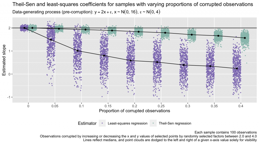
The Theil-Sen estimator handles the injection of extremity into the data far better than the least-squares estimator. In this simulation, by the time 20% of the points in each sample are corrupted, the point cloud of least-squares estimates entirely excludes 2.0 (the true slope of the data-generating process for the uncorrupted data). For any given proportion of corrupted data points, the Theil-Sen estimates also exhibit less variance sample to sample than the least-squares estimates. At, for example, a corrupted-data proportion of 0.15, the bundle of Theil-Sen estimates, although no longer centered around 2.0, hews fairly close to that value and has limited dispersion. The least-squares estimates behave much more erratically, exhibiting large, unpredictable divergences from 2.0. (Formally, the Theil-Sen estimator has a breakdown point of 29.3%, meaning that it can tolerate the corruption of 29.3% of the input data before the slope estimate can become arbitrarily large in magnitude; Rousseeuw & Leroy, 1987, see p. 9 and p. 67.)

Confidence intervals for the slope and intercept estimates can be derived via bootstrapping. One generates B bootstrap samples by resampling the original data with replacement; each of the B replicates contains n observations, where n is the number of points in the original data. From there, one calculates Theil-Sen slope and intercept estimates for each bootstrap sample, and confidence intervals can be estimated by taking the \(\alpha/2\) and \(1 - (\alpha/2)\) quantiles of the bootstrapped values, where \(\alpha = 100\% - CI\%\) (Wilcox, 1998; Wilcox, 2001, pp. 208–209).

# Simulate data
x <- rnorm(50, 0, 4)
y <- 2 + 4*x + rnorm(50, 0, 1)
dat <- data.frame(x, y)

# Bootstrap
b <- 2500
boot_theil_sen <- function(dat) {
  boot_dat <- dat[sample(nrow(dat), replace = T), ]
  theil_sen(boot_dat)
}
boots <- data.frame(t(replicate(b, boot_theil_sen(dat))))

# Percentile-based bootstrap 95% confidence intervals
# Theil-Sen intercept
quantile(boots[, grep(x = colnames(boots), pattern = 'intercept')], probs = c(.025, .975))

    2.5%    97.5% 
1.609699 2.277515 

# Theil-Sen slope
quantile(boots[, grep(x = colnames(boots), pattern = 'slope')], probs = c(.025, .975))

    2.5%    97.5% 
3.909880 4.078623 

The simulation results in this piece are a fine advertisement for Theil-Sen regression. That said, the simulation intentionally investigated conditions that provoke poor performance on the part of least squares. The natural question, then, is: In the wild, when the properties of the data are the very thing being investigated, not the thing being simulated, when should one consider Theil-Sen regression instead of least squares?

When estimating a linear relationship, Theil-Sen (or another robust regression method¹) is advantageous if outliers are a known, discovered, or suspected risk. Under conditions optimized for least squares (no outliers; normally distributed least-squares residuals; homogeneous residual variance), least squares has a slight advantage over Theil-Sen in terms of the width of coefficient standard errors (and corresponding confidence intervals), but the edge is minimal. And as the parametric assumptions of least squares break down—a common occurrence in practice—least-squares standard errors can shoot up to be hundreds of times larger than corresponding values from Theil-Sen regression (see Wilcox, 1998, for a slate of comparative results). Consider too the results from the simulation above for samples containing no corrupted points (in which residuals were normally distributed and had homogeneous variance): The accuracy and spread of the Theil-Sen estimates was functionally identical to that of the least-squares estimates.

At large sample sizes, calculating a Theil-Sen regression can have a high computational cost, as one needs to calculate as many as \(n(n-1)/2\) slopes (e.g., \(10,000(10,000-1)/2 = 49,995,000\)). This can be a frustration when n is extreme,² but modern computers are hearty machines ready to handle intensive computations with reasonable speed and dignity. And the time saved up-front by estimating a least-squares regression can be lost on the back-end by follow-up outlier detection and assessment of the model’s fragility.

Universal recommendations are hard to offer or come by in applied statistics, and I won’t make one here. (Universal proscriptions seem more forthcoming!) But for assessments of bivariate linear relationships in data that are outlier-infested, I’m motivated to consider alternatives to least squares. Removing extreme points from a data set to facilitate least-squares regression rightfully raises alarm bells—it’s difficult to justify removal unless an observation can be identified as literally erroneous—and Theil-Sen regression’s resistance to outlier-induced instability and inaccuracy in slope estimates makes it an appealing option.

References

• Rousseeuw, P. J., & Leroy, A. M. (1987). Robust regression and outlier detection. Wiley.
• Sen, P. K. (1968). Estimates of the regression coefficient based on Kendall’s tau. Journal of the American Statistical Association, 63(324), 1379–1389. https://doi.org/10.2307/2285891
• Siegel, A. F. (1982), Robust regression using repeated medians. Biometrika, 69(1), 242–244. https://doi.org/10.1093/biomet/69.1.242
• Theil, H. (1950). A rank-invariant method of linear and polynomial regression analysis. Proceedings of the Royal Netherlands Academy of Sciences, 53, 368–392 (Part I), 521-525 (Part II), 1397-1412 (Part III).
• Wilcox, R. R. (1998). A note on the Theil‐Sen regression estimator when the regressor is random and the error term is heteroscedastic. Biometrical Journal, 40(3), 261–268. https://doi.org/10.1002/(SICI)1521-4036(199807)40:3%3C261::AID-BIMJ261%3E3.0.CO;2-V
• Wilcox, R. R. (2001). Fundamentals of modern statistical methods: Substantially improving power and accuracy (1st ed.). Springer. https://doi.org/10.1007/978-1-4757-3522-2
• Young, D. S. (2017). Handbook of regression methods. Chapman and Hall/CRC. https://doi.org/10.1201/9781315154701

Jacob Goldstein-Greenwood
Research Data Scientist
University of Virginia Library
April 28, 2023

Appendix: Theil-Sen estimators on CRAN, and the behavior of mblm::mblm() (version 0.12.1) in the presence of NA values

At least four R packages on CRAN provide functions for Theil-Sen regression: deming; mblm; robslopes; and RobustLinearReg.

In preparing this article, I found that mblm::mblm() (version 0.12.1), which calculates a Theil-Sen slope and intercept, does not appear to behave reliably when NA values are in the input data:

Given vectors x and y (containing the x and y values for each observation), mblm::mblm() first applies a sort() function to x, saving the sorted result as xx. The function then sorts y by the original order of x, saving the result as yy. This works without issue if x and y have no NA values, but if x contains an NA value, the value is dropped by sort(). When y is then sorted by the order of x (i.e., y[order(x)]), the resulting vectors—xx and yy—differ in length, as the value of y corresponding to the missing value of x is shunted to the end of the ordered yy vector, not dropped. When the Theil-Sen intercept is calculated later in the function via the code yy - slope * xx (where slope is the Theil-Sen slope estimate), that difference in vector lengths results in a value of the now-shorter xx object being recycled during the calculation of the intercept for each point. Conversely, if x is complete but y has one or more missing values, x is sorted into xx without issue, but the NA values in y are retained in the ordered yy vector. Downstream, this means that NA values wind up in the vectors of point-to-point slopes and single-point intercepts from which the Theil-Sen slope and intercept are calculated, and the function output becomes NA for both values. I show this behavior below, and the source code for version 0.12.1 can be found on GitHub at this link. As of the time I write this, the mblm package hasn’t been updated on CRAN since 2019, so I’m not holding my breath for a fix.

NA_x <- data.frame(x = c(2, 4, NA, 1),
                   y =- c(3, 2.5, 3, 1))
NA_y <- data.frame(x = c(2, 4, 3, 1),
                   y =- c(3, 2.5, NA, 1))
no_NA <- na.omit(NA_x)

# mblm() Theil-Sen estimate when only complete cases are used
mblm::mblm(y ~ x, no_NA, repeated = FALSE)

Call:
mblm::mblm(formula = y ~ x, dataframe = no_NA, repeated = FALSE)

Coefficients:
(Intercept)            x  
       -0.5         -0.5  

# mblm() Theil-Sen estimate when x contains an NA value
# (Note that a warning is produced hinting at the recycling of x values)
mblm::mblm(y ~ x, NA_x, repeated = FALSE)

Warning in yy - slope * xx: longer object length is not a multiple of shorter
object length

Call:
mblm::mblm(formula = y ~ x, dataframe = NA_x, repeated = FALSE)

Coefficients:
(Intercept)            x  
      -1.25        -0.50  

# mblm() Theil-Sen estimate when y contains an NA value
mblm::mblm(y ~ x, NA_y, repeated = FALSE)

Call:
mblm::mblm(formula = y ~ x, dataframe = NA_y, repeated = FALSE)

Coefficients:
(Intercept)            x  
         NA           NA