
Analysts and researchers occasionally want to compare the magnitudes of different predictive or causal effects estimated via regression. But comparison is a tricky endeavor when predictor variables are measured on different scales: If y is predicted from x and z, with x measured in kilograms and z measured in years, what does the relative size of the variables’ regression coefficients communicate about which variable is “more strongly” associated with y?
Standardized regression coefficients, which express the average change in standard deviations of an outcome variable associated with a one-standard-deviation change in a predictor variable, are advertised by various statistical sources as a solution to the challenge of comparison. The SAGE Encyclopedia of Social Science Research Methods, published in 2004, lauds standardized coefficients with the following language:
…when independent variables are measured in different units (for example, years of schooling for one variable, IQ score for another, etc.), it is difficult, based only on the unstandardized coefficients, to discern which of two or more independent variables has more impact on the dependent variable. … Using standardized coefficients converts all of the coefficients to a common unit of measurement (standard deviations), and the standardized coefficient is the same regardless of the units in which the variable was originally measured. A larger standardized coefficient for one independent variable as opposed to a second independent variable allows us to conclude that the first independent variable has a stronger influence than the second independent variable, even when the two independent variables were originally measured in very different units.
The premise—one I’ll happily denigrate here—is that standardized coefficients can be used to assess the relative magnitudes of effect sizes within or across studies: One is purportedly able to compare coefficients on a shared, unitless scale: “A one-standard-deviation change in x is associated with a half-standard-deviation change in y, but a one-standard-deviation change in z is associated with a one-standard-deviation change in y; the predictive effect of z must be far larger than that of x.”
But these tweaked measures of association have been the subject of earned attacks for decades (e.g., Blalock, 1961; Greenland et al., 1986; Greenland et al., 1991, King, 1986). The Achilles’ heel of standardized coefficients—it’s a sufficiently serious issue that we could plausibly call it an Achilles’ torso—is that they confound estimates of the relationships between variables with the sample variances thereof. (Despite this, even some relatively recent books on regression frame standardized coefficients as trustworthy comparative tools; e.g., Freund and Wilson [2003]: “Comparison of coefficients across variables can be made by the use of standardized coefficients” [p. 350].1)
The equation for calculating standardized coefficients makes explicit the dependence of the standardized estimate on the sample variances of the variables involved: An unstandardized coefficient is multiplied by the standard deviation of predictor x (\(s_x\)) and divided by the standard deviation of outcome y (\(s_y\)). (The calculation sometimes omits the divide-by-\(s_y\) step, in which case the standardized coefficient reflects the change in units of y associated with a one-standard-deviation change in x. The issues I discuss here are relevant to standardized coefficients calculated by either method. Note too that standardized coefficients can be alternatively calculated by first z-scoring—standardizing—the predictor and, optionally, the outcome variable and then estimating a regression between the transformed variables.)
\[\hat{\beta}^* = \hat{\beta}\frac{s_x}{s_y}\]
Comparisons of different predictors’ standardized coefficients, or comparisons of coefficient estimates for a single predictor calculated in different studies or among different populations, are rendered suspect because an observed difference in standardized coefficients could either be due to an actual difference in the magnitude of the underlying relationships being estimated or be due to differences in the standard deviations of the involved variables.
I demonstrate this problem in the simulation below. I repeatedly sample x, y, and z from each of two populations; in both, y is a linear function of x and z. My aim is to estimate and compare the relationship between x and y across populations. Critically, the true relationship between x and y is identical in both populations: A one-unit increase in x is associated with a two-unit increase in y (i.e., unstandardized β = 2.0). However, the standard deviation of x varies: In population 1, it’s 5.0; in population 2, it’s 9.0. (In both populations, the true relationship between z and y is β = 2.0, and the standard deviation of z, \(\sigma_z\), is 7.0.) In each sample, I estimate a linear regression predicting y from x and z. I then standardize the coefficient of x in two ways: First, by multiplying the raw coefficient by \(s_x\), and second, by multiplying it by \(\frac{s_x}{s_y}\). I repeat this process 250 times at each of several sample sizes. The standardized coefficients are plotted below.
set.seed(999)
ns <- seq(25, 250, by = 25)
times <- 250
# x1, z1, y1 are from population 1; x2, z2, y2 are from population 2
calc_coefs_x <- function(n, x1_sd, x2_sd, x1_b, x2_b, z_sd, z_b) {
  x1 <- rnorm(n, mean = 0, sd = x1_sd); x2 <- rnorm(n, mean = 0, sd = x2_sd)
  z1 <- rnorm(n, mean = 0, sd = z_sd); z2 <- rnorm(n, mean = 0, sd = z_sd)
  y1 <- x1_b*x1 + z_b*z1 + rnorm(n, 0, 1); y2 <- x2_b*x2 + z_b*z2 + rnorm(n, 0, 1)
  coef1 <- coef(lm(y1 ~ x1 + z1))[['x1']]; coef2 <- coef(lm(y2 ~ x2 + z2))[['x2']]
  c('coef1_sx' = coef1*sd(x1), 'coef2_sx' = coef2*sd(x2),
    'coef1_sxsy' = coef1*(sd(x1)/sd(y1)), 'coef2_sxsy' = coef2*(sd(x2)/sd(y2)))
}
out <- vector(mode = 'list', length = length(ns))
for (i in 1:length(ns)) {
  tmp <- replicate(times, calc_coefs_x(n = ns[i], x1_sd = 5, x2_sd = 9, x1_b = 2, x2_b = 2,
                                       z_sd = 7, z_b = 2))
  tmp <- data.frame(t(tmp)); tmp$n <- ns[i]; out[[i]] <- tmp
}
out <- data.table::rbindlist(out)
out <- tidyr::pivot_longer(out, cols = -n, names_to = c('pop', 'standardized_via'),
                           names_pattern = 'coef(\\d)_(.+)', values_to = 'beta')
lab <- expression(paste(atop(paste('True data-generating process in population 1: ',
                                   y == 2*x + 2*z + epsilon, ', ', x %~% N(0, 25), ', ',
                                   z %~% N(0, 49), ', ', epsilon %~% N(0, 1)),
                             paste('True data-generating process in population 2: ',
                                   y == 2*x + 2*z + epsilon, ', ', x %~% N(0, 81), ', ',
                                   z %~% N(0, 49), ', ', epsilon %~% N(0, 1)))))
out$standardized_via <- factor(out$standardized_via, levels = c('sx', 'sxsy'),
                               labels = c(
                                 expression(paste('Standardized via: ', beta %*% s[x])),
                                 expression(paste('Standardized via: ', beta %*% (s[x]/s[y]))))
                               )
medians <- aggregate(out$beta, by = list(out$n, out$pop, out$standardized_via), median)
colnames(medians) <- c('n', 'pop', 'standardized_via', 'beta')
library(ggplot2)
ggplot(out, aes(x = n, y = beta, color = pop)) +
  geom_jitter(width = 5) +
  geom_line(data = medians, aes(x = n, y = beta, group = pop, linetype = pop), color = 'black') +
  facet_wrap(~ standardized_via, scales = 'free', labeller = label_parsed) +
  labs(title = 'Standardized coefficient of x across sample sizes',
       subtitle = lab, y = 'Standardized coefficient value',
       color = 'Population', linetype = 'Population',
       caption = 'Lines reflect the median value in each population at each sample size') +
  scale_color_manual(values = c('cornflowerblue', 'salmon')) +
  scale_linetype_manual(values = c("dashed", "dotted")) +
  theme(legend.position = 'bottom')
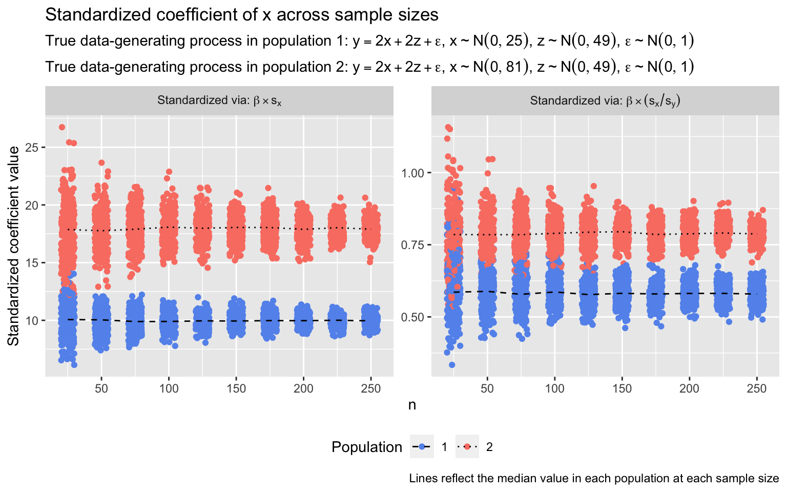
The conclusion one would draw from either set of standardized coefficients is that the relationship between x and y in population 2 is far larger than the relationship in population 1. This would be an offense to verity: The relationships are identical in both populations. Increasing the sample size addresses nothing but the stability of the standardized coefficient estimates: The coefficients are estimated more precisely at larger sample sizes, but the inaccuracy of the conclusion the coefficients suggest is as serious when \(n = 250\) as when \(n = 25\). (The ratio of median standardized coefficients differs between populations depending on whether or not standardization includes the divide-by-\(s_y\) step because the standard deviation of y—as a joint function of x and z—also differs between populations.)
Or consider a different but similarly egregious case, one in which the relationship between x and y (which is still a linear function of x and z) does vary between populations, but due to differences in the variance of x in each population, standardized coefficients suggest that the direction of the difference in effect magnitudes across populations is the reverse of what it actually is. Below, I conduct a simulation similar to the previous one, except that now:
- In population 1, x has a standard deviation of 9.0
- In population 2, x has a standard deviation of 4.0
- In population 1, the true (unstandardized) relationship between x and y is β = 1.0
- In population 2, the true (unstandardized) relationship between x and y is β = 2.0
- (For z, β and \(\sigma_z\) are again 2.0 and 7.0, respectively, in both populations)
out <- vector(mode = 'list', length = length(ns))
for (i in 1:length(ns)) {
  tmp <- replicate(times, calc_coefs_x(n = ns[i], x1_sd = 9, x2_sd = 4, x1_b = 1, x2_b = 2,
                                       z_sd = 7, z_b = 2))
  tmp <- data.frame(t(tmp)); tmp$n <- ns[i]; out[[i]] <- tmp
}
out <- data.table::rbindlist(out)
out <- tidyr::pivot_longer(out, cols = -n, names_to = c('pop', 'standardized_via'),
                           names_pattern = 'coef(\\d)_(.+)', values_to = 'beta')
lab <- expression(paste(atop(paste('True data-generating process in population 1: ',
                                   y == 1*x + 2*z + epsilon, ', ', x %~% N(0, 81), ', ',
                                   z %~% N(0, 49), ', ', epsilon %~% N(0, 1)),
                             paste('True data-generating process in population 2: ',
                                   y == 2*x + 2*z + epsilon, ', ', x %~% N(0, 16), ', ',
                                   z %~% N(0, 49), ', ', epsilon %~% N(0, 1)))))
out$standardized_via <- factor(out$standardized_via, levels = c('sx', 'sxsy'),
                               labels = c(
                                 expression(paste('Standardized via: ', beta %*% s[x])),
                                 expression(paste('Standardized via: ', beta %*% (s[x]/s[y]))))
                               )
medians <- aggregate(out$beta, by = list(out$n, out$pop, out$standardized_via), median)
colnames(medians) <- c('n', 'pop', 'standardized_via', 'beta')
ggplot(out, aes(x = n, y = beta, color = pop)) +
  geom_jitter(width = 5) +
  geom_line(data = medians, aes(x = n, y = beta, group = pop, linetype = pop), color = 'black') +
  facet_wrap(~ standardized_via, scales = 'free', labeller = label_parsed) +
  labs(title = 'Standardized coefficient of x across sample sizes',
       subtitle = lab, y = 'Standardized coefficient value',
       color = 'Population', linetype = 'Population',
       caption = 'Lines reflect the median value in each population at each sample size') +
  scale_color_manual(values = c('cornflowerblue', 'salmon')) +
  scale_linetype_manual(values = c("dashed", "dotted")) +
  theme(legend.position = 'bottom')
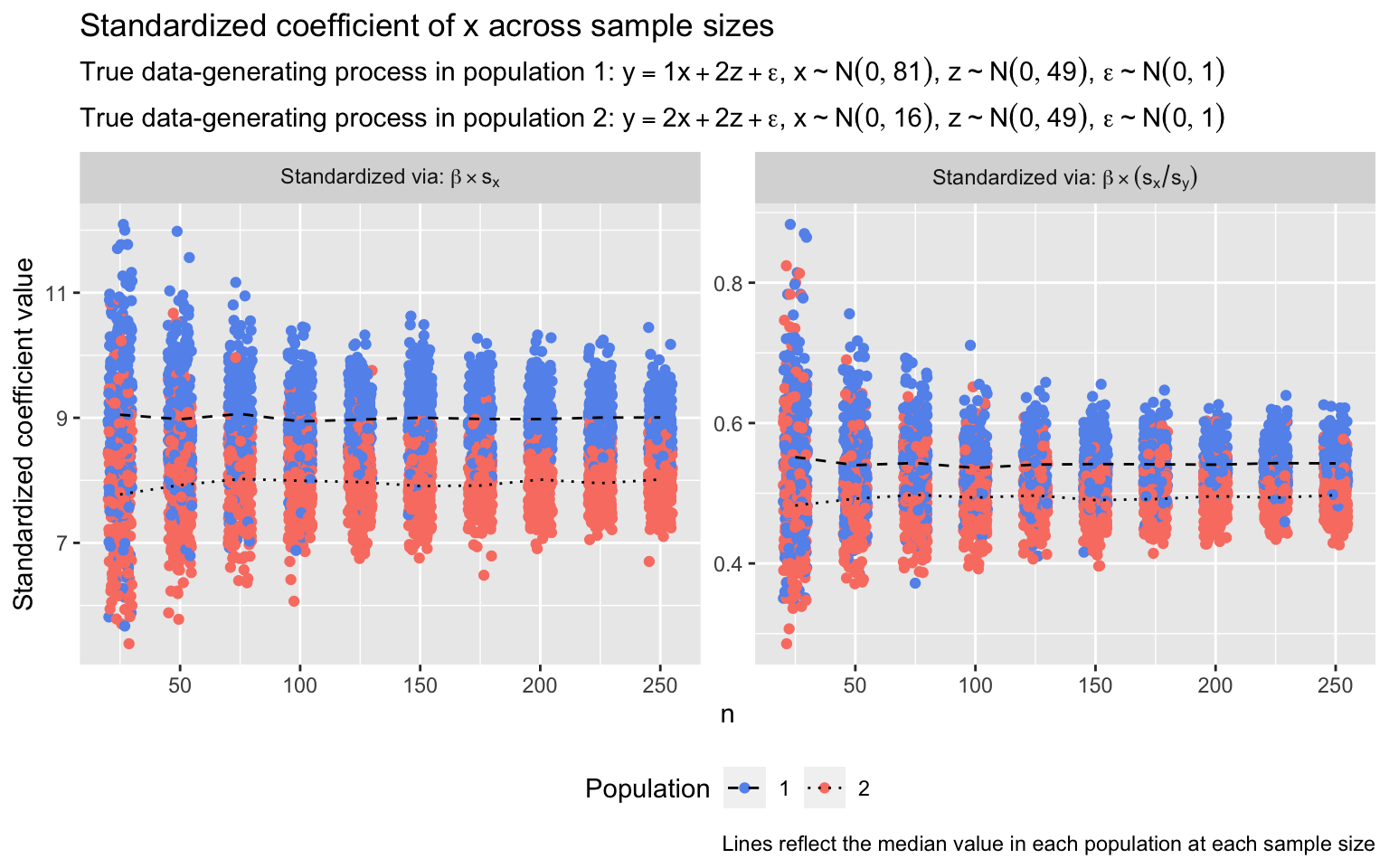
With the standard deviation of x in population 1 exceeding that in population 2, the standardized coefficients are contorted to such a degree that they make the magnitude of the relationship between x and y appear larger in population 1 than in population 2, despite the relationship being, in truth, twice as large in population 2.
The simulations above exemplify the misleading effects of coefficient standardization via comparisons of effect magnitudes across studies. The issues are similarly serious for within-study comparisons of predictor effects. When predicting, say, y jointly from x and z, the standardized coefficient for each predictor is in no small part determined by the variable’s sampling variance (and by the distribution of the outcome if standardization involves division by \(s_y\)).
Notable too is that the examples above all involve predictors that are on the same scale: The same (imaginary) variable, x, is measured in two different populations. Standardization mangles my ability to reliably compare predictive effects in cases where I could have compared unstandardized coefficients without issue. I’ll quote John Fox and Sanford Weisberg: “If standardization distorts coefficient comparisons when the predictors have the same units, in what sense does standardization allow us to compare coefficients of predictors that are measured in different units, which is the dubious application to which standardized coefficients are often put?” (2019, p. 187).
Further troubling is the fact that variables’ sample standard deviations result in no small part from features of study design—sometimes arbitrary features, at that. In a 1991 paper discussing standardized coefficients’ propensity to mislead, Sander Greenland and colleagues describe two studies that examined the relationship between cholesterol and coronary heart disease using logistic regressions, the Pooling Project and the Honolulu Heart Study. The samples included in each study’s analysis differed in ways that were bound to influence the sample variance of key variables: “…only subjects aged 40–59 at the start of follow-up were included [in the Pooling Project’s analysis]. …most of the Honolulu Heart Study subjects were aged 60–75…” (pp. 387–388). Insofar as age and cholesterol are related, the distinct age ranges of the samples mean that the standard deviation of cholesterol can hardly be expected to remain constant (or close to it) across them. Logistic regression coefficients characterizing the association between cholesterol and coronary heart disease are rendered less comparable, not more, by standardization. This problem embeds itself in any situation in which differences in study design open the door to fickle aberrations in variables’ standard deviations.
If standardizing a regression coefficient improves the interpretability of a model—because the predictor (and optionally outcome) involved can be sensibly thought about in terms of standard deviations—standardize away.2 Doing so can be as reasonable as putting “annual revenue” in terms of millions of dollars or “city population” in terms of thousands of people. Trouble arises when standardized coefficients are taken as globally valid means of effect-size comparison. The notion that a standard deviation of a is inherently comparable to a standard deviation of b is illusory.
R session details
The analysis was done using the R Statistical language (v4.5.2; R Core Team, 2025) on Windows 11 x64, using the packages ggplot2 (v4.0.1).
References
- Blalock, H. M., Jr. (1961). Evaluating the relative importance of variables. American Sociological Review 26(6), 866–874.
- Fox, J., & Weisberg, S. (2011). An R companion to applied regression (2nd ed.). SAGE.
- Fox, J., & Weisberg, S. (2019). An R companion to applied regression (3rd ed.). SAGE.
- Freund, R. J., & Wilson, W. J. (2003). Statistical methods. Elsevier.
- Greenland, S., Maclure, M., Schlesselman, J. J., Poole, C., & Morgenstern, H. (1991). Standardized regression coefficients: A further critique and review of some alternatives. Epidemiology, 2(5), 387–392.
- Greenland S., Schlesselman, J. J., & Criqui, M. H. (1986). The fallacy of employing standardized regression coefficients and correlations as measures of effect. American Journal of Epidemiology, 123(2), 203–208.
- King, G. (1986). How not to lie with statistics: Avoiding common mistakes in quantitative political science. American Journal of Political Science, 30(3), 666–687.
- Menard, S. (2004). Standardized regression coefficients. In M. S. Lewis-Beck, A. Bryman, & T. F. Liao (Eds.), The SAGE encyclopedia of social science research methods. SAGE.
Jacob Goldstein-Greenwood
Research Data Scientist
University of Virginia Library
March 9, 2023
- Plenty of modern textbooks are not so sympathetic. The second edition of Fox and Weisberg’s An R Companion to Applied Regression (2011) notes that “[u]sing standardized predictors apparently permits comparing regression coefficients for different predictors, but this is an interpretation that we believe does not stand up to scrutiny” (p. 184). The third edition of their book (2019) likens coefficient standardization to using an “elastic ruler” (p. 187). ↩︎
- However, Greenland et al. (1991) point out that as far as measures of variation one could use to standardize coefficients go, the standard deviation is not necessarily optimal: Measures like the interquartile range and median absolute deviation provide a more-intuitive sense of distributional variation when working with non-normal variables. ↩︎
For questions or clarifications regarding this article, contact statlab@virginia.edu.
View the entire collection of UVA Library StatLab articles, or learn how to cite.