The Intuition Behind Confidence Intervals

Say it with me: An X% confidence interval captures the population parameter in X% of repeated samples.

In the course of our statistical educations, many of us had that line (or some variant of it) crammed, wedged, stuffed, and shoved into our skulls until definitional precision was leaking out of noses and pooling on our upper lips like prop blood.

Or, at least, I felt that way.

But hearing the line over and over didn’t do a lot to make it any more intuitive. And that’s no surprise: Confidence intervals are an odd concept, and without the right blend of prose and pictures, it can be difficult to “get” the intuition. This piece is a brief attempt to build, from the ground up, the intuition behind (frequentist) confidence intervals through a simple example.

The world of coffee is infused with delightful disagreement: For any given brewing method, people go back and forth about how much ground coffee to use, how much water to use, how hot that water should be, how long the brew process should take, and so on.

Personally, I’m partial to making coffee with an AeroPress. For the unfamiliar, the AeroPress is a simple, manually operated, cylindrical coffeemaker. A person steeps grounds and hot water together before pressing coffee out of the cylinder into a cup using a plunger.

aeropress coffee maker
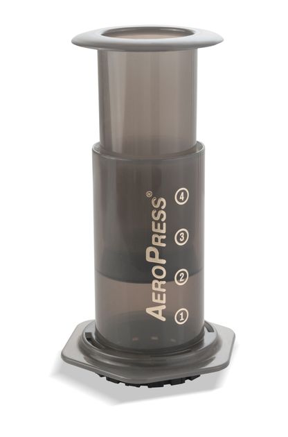
Photo: Kimi Boi. Source. Used under a CC BY-SA 4.0 license.

These days, I use around 11.5 grams of ground coffee and 225 grams of water in my AeroPress. But I’m curious about how that compares to other AeroPress users. Say that I want to estimate the average amount of ground coffee, in grams, that members of an online coffee forum use when brewing with an AeroPress. And say that the forum has around 20,000 members (which is not far off from the number of members that the subreddit dedicated to the AeroPress has as of October 2021). With enough resources and time, perhaps I could survey every forum member and calculate the average based on all relevant data points. The average calculated in that case would be perfectly accurate and errorless. But surveying 20,000 people is rarely realistic. Instead, to estimate the “population” (forum-wide) average, I’d need to take a random sample of forum members and base the estimate on that. However, if I take a sample of, say, 100 people and calculate the sample mean, I’m likely to get a value that differs somewhat from the true mean (the average across all 20,000 people): If the forum-wide mean is 12.52 grams, I might get a sample mean of 12.34, 12.22, or perhaps 13.00. The sample mean will have some sampling error associated with it. To try and account for some of that sampling error, I’d like to calculate a range around whatever sample mean I obtain—a confidence interval—that, hopefully, captures the true mean with some degree of reliability.

To build the intuition behind confidence intervals, let’s pretend for a moment that we have access to the measures for all 20,000 hypothetical people. The distribution of grams of coffee used across all forum members might look something like this:


library(ggplot2)
set.seed(2021)
coffee <- data.frame(grams = c(rnorm(12500, 12.5, 2), runif(7500, 10, 15)))
coffee$grams <- ifelse(coffee$grams < 8, 8, coffee$grams)
ggplot(coffee, aes(x = grams)) +
  geom_histogram(fill = 'cadetblue', bins = 50) +
  geom_vline(xintercept = mean(coffee$grams), color = 'gold') +
  labs(title = 'Distribution of Grams of Coffee Used Across All 20,000 Forum Members',
       y = 'Number of People', x = 'Grams of Coffee')

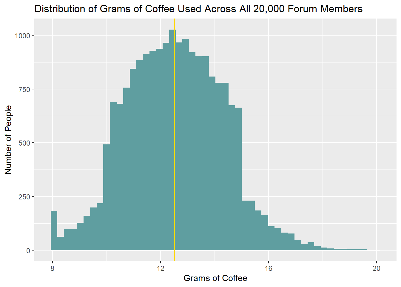
distribution of grams of coffee used across all forum members, faux data

In the simulated distribution above, the true mean among all forum members is 12.52 grams, and the standard deviation is 1.80 grams.

\(\mu = 12.52\ grams\)
\(\sigma = 1.80\ grams\)

The intuition

If we were to draw random samples of a given size—say, 100 people—from the coffee forum over and over and calculate a sample mean each time, we’d build up a distribution of sample means: a sampling distribution. Critically, the sampling distribution would be centered on the population mean, and it would approximate a normal distribution, regardless of whether the underlying values in the population are themselves normally distributed (this is the central limit theorem). Further, the sampling distribution would have a standard deviation given by the formula below—this is the standard error of the sampling distribution:

\(SE = \frac{\sigma}{\sqrt{n}}\)

\(\sigma\): Standard deviation of values in the population
\(n\): Sample size

(To catch the intuition behind this formula, consider that: (1) As the standard deviation of values in the population, \(\sigma\), increases, the width of the sampling distribution increases because more variability in population values means more variability in sample means; and (2) as n increases, each sample better approximates the population, reducing variability in sample means.)

Note that we rarely know \(\sigma\), and we generally have to estimate it using the standard deviation of the sample. (More on this below under The practical calculation.)

If we were to endlessly draw random samples with \(n = 100\) from the simulated coffee data (which has \(\mu = 12.52\) and \(\sigma = 1.80\)) and calculate the sample mean each time, we’d build up a normal distribution of sample means that looks like so:

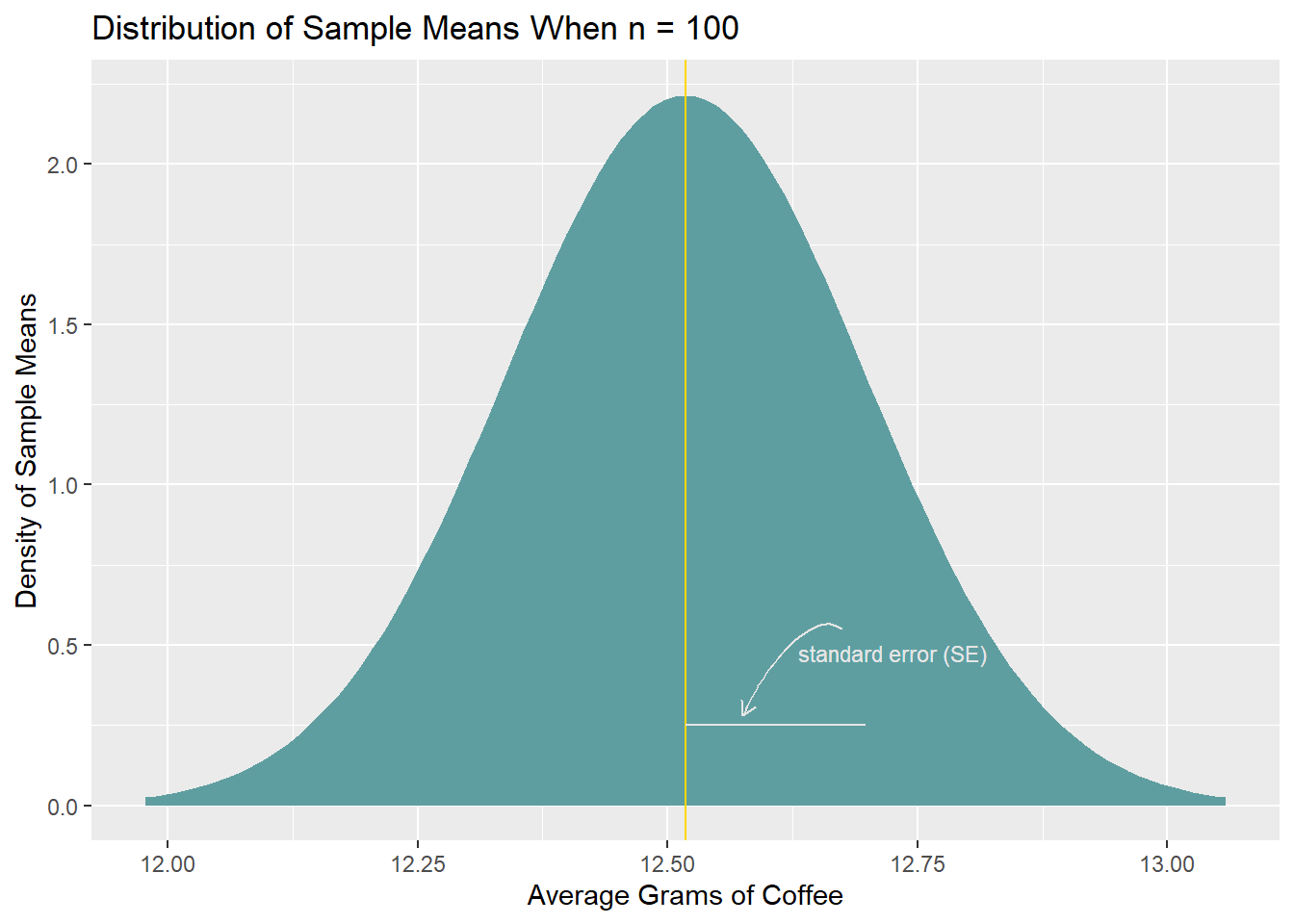
sampling distribution of average grams of coffee used, n = 100 per sample, with standard error superimposed

We can find an interval in this sampling distribution, centered around its mean (the gold line), that captures a certain percentage of the sample means. We’ll pick 95%. (The selection of 95% is ultimately arbitrary. There’s no particular justification for picking 95% instead of 94%, 91%, 99%, etc.; 95% is simply a custom, a default, that many people reach for.)

To determine the interval, we find the points in the distribution below which 2.5% and 97.5% of the values fall (i.e., the points that capture the inner 95% of the data). In a normal distribution, those quantiles occur 1.96 standard deviations below and above the mean, respectively. We can therefore calculate the quantiles by taking \(mean - (1.96 * SE)\) and \(mean + (1.96 * SE)\). (As a terminological reminder, an SE/standard error is a standard deviation of a sampling distribution.)

Here, in the theoretical sampling distribution with \(\mu = 12.52\) and \(SE = \frac{\sigma}{\sqrt{n}} = \frac{1.80}{\sqrt{100}} = 0.18\), the interval ranges from 12.16 to 12.87.


# Manually calculate population SD, as sd() function divides by n - 1 instead of n
pop_sd <- sqrt(sum((coffee$grams - mean(coffee$grams))^2) / nrow(coffee))
# Note that 12.52 and 0.18 are the rounded mean and SE
se <- pop_sd / sqrt(100)
lo <- mean(coffee$grams) - (1.96 * se)
hi <- mean(coffee$grams) + (1.96 * se)
interval <- c(lo, hi)
interval


[1] 12.16489 12.87077


# Or, shortcut the steps above with:
# interval <- qnorm(c(.025, .975), mean = mean(coffee$grams), sd = (pop_sd / sqrt(100)))

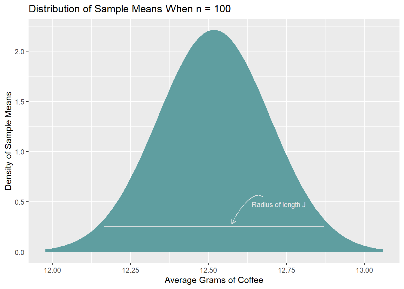
sampling distribution of average grams of coffee used, n = 100 per sample, with confidence interval superimposed at center of distribution

This interval has a radius of length J (the distance from the gold line to the end of one side of the interval; one half of the full interval width). Consider what would happen if we were to take this interval and place it around every sample mean in the sampling distribution: For sample means that lie \(\le J\) from the center of the sampling distribution, the interval would capture the population mean. The only sample means that lie \(> J\) from the center of the distribution are in the bottom 2.5% and top 2.5% of the sampling distribution.

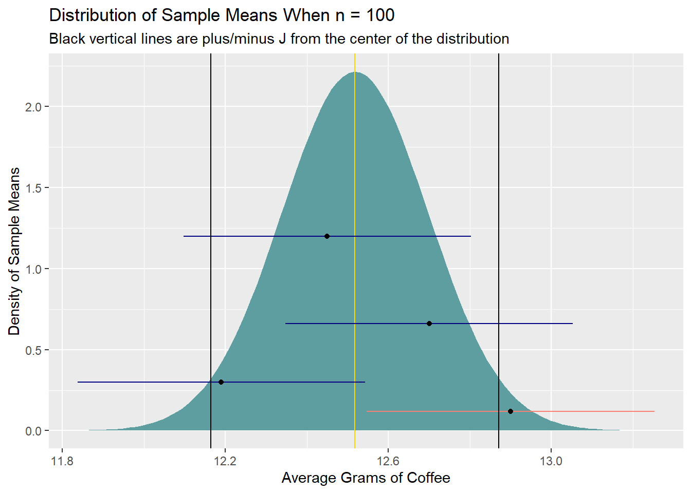
sampling distribution of average grams of coffee used, n = 100 per sample, with several confidence intervals superimposed around various sample means

The sampling distribution contains the possible means one might obtain when drawing samples of a particular size from the population. We can say, then, that this interval—the 95% confidence interval—will capture the population mean in 95% of repeated samples of size \(n\) if placed around the sample means. This is the core intuition behind frequentist confidence intervals: If you can decently estimate J, you can find an interval that would capture the population mean when dropped around the sample mean in some set percentage of repeated samples.

Of course, in any given study/experiment/etc., we generally only take one sample, and we can’t know if the sample mean’s distance from the center of the sampling distribution is indeed \(\le J\). But we can have a certain level of confidence in the process by which we generate the interval. (This is a key point, and it’s one worth reiterating: Our confidence is in the interval-generation process, not in any specific interval itself. It doesn’t follow from the way frequentist confidence intervals are calculated that “there’s a 95% chance that the 95% confidence interval contains the population parameter.” Once the interval is calculated, it either captures the population parameter or does not.)

The practical calculation

Our goal, then, when we take a sample and calculate a sample mean, \(\bar{x}\), is to find J, the radius, which allows us to calculate the confidence interval as \([\bar{x} - J, \bar{x} + J]\).

Finding the radius is equivalent to traveling a certain number of standard deviations (standard errors) out from the center of the sampling distribution. We don’t know where the center of the sampling distribution is, but that’s not an issue: The width of the sampling distribution depends on the standard deviation of the population values, not on the population mean.

If we know the population standard deviation, we can exactly calculate the standard error of the sampling distribution as:

\(SE_{\sigma\ known} = \frac{\sigma}{\sqrt{N}}\).

And, as mentioned above, in a normal distribution, the 2.5% and 97.5% quantiles occur 1.96 standard deviations below and above the sampling distribution mean, thus allowing us to calculate the radius of the 95% confidence interval, J, as:

\(J_{\sigma\ known} = 1.96 * \frac{\sigma}{\sqrt{n}}\)

However, almost never do we know the population standard deviation. When the population standard deviation is unknown, we estimate it with the sample standard deviation, \(s\), and we plug that value in when estimating the standard error of the sampling distribution:¹

\(SE_{\sigma\ unknown} = \frac{s}{\sqrt{n}}\)

Further, when the population standard deviation is unknown, instead of using a normal distribution to estimate the number of standard errors that the 2.5% and 97.5% quantiles lie away from the center of the sampling distribution, we use a t distribution with \(n - 1\) degrees of freedom. (Think of using a t distribution here as a partial prophylactic against underestimating the confidence interval: Although “normal-ish,” the exact shape of the t distribution depends on the sample size, and relative to a normal curve, the t distribution has fatter tails, particularly for small sample sizes.²) As it’s generally necessary to use \(s\) instead of \(\sigma\), we usually calculate the radius of the 95% confidence interval of the mean as:

\(J_{\sigma\ unknown} = t_{0.975,\ n-1}^* * \frac{s}{\sqrt{n}}\)

\(t^*\) is the 97.5% quantile of a t distribution with \(n-1\) degrees of freedom
\(s\) is the sample standard deviation
\(n\) is the sample size

With J in hand, we can then calculate the confidence interval of the mean as \([\bar{x} - J, \bar{x} + J]\).

Note too that for relatively large sample sizes, the value that one multiplies the standard error by will be effectively identical regardless of whether calculated using a normal distribution or a t distribution:

Distribution	2.5% quantile	97.5% quantile	Degrees of freedom
Standard normal	-1.960	1.960	NA
t	-1.984	1.984	99
t	-1.962	1.962	999
t	-1.960	1.960	9999

Back to the AeroPress example

Having developed the intuition behind why an X% confidence interval captures the population parameter in X% of repeated samples, I’ll return to the case of estimating the average number of grams of coffee that people on an online forum use when preparing coffee with an AeroPress.

Assume that I know neither the population mean nor the population standard deviation. I instead draw a random sample of \(n = 100\) from the population data simulated at the top of this article and calculate a 95% confidence interval around the sample mean.

The sample mean, \(\bar{x}\), is:


coffee_sample <- sample(coffee$grams, 100, replace = F)
mean(coffee_sample)


[1] 12.61863

To calculate the confidence interval, I need to estimate the standard error, which, lacking the population standard deviation, I’ll base on the sample standard deviation, \(s\):


SE <- sd(coffee_sample) / sqrt(100) # The sd() call uses a denominator of n-1; see footnote 1
SE


[1] 0.1741082

From here, I need to determine how many standard errors away from the center of the theoretical sampling distribution I’d need to travel in each direction to capture 95% of the values therein. As I don’t know the standard deviation of values in the population and had to plug in the sample standard deviation (\(s\)) as an estimator, I’ll determine the number of standard errors by which I need to multiply \(s\) by considering a \(t\) distribution with \(n - 1 = 99\) degrees of freedom.


# Note that it's only technically necessary to calculate this for the 97.5% quantile
# (The 2.5% quantile is simply the negative of the 97.5% quantile)
num_SEs <- qt(0.975, df = 99)
num_SEs


[1] 1.984217

I’ve now estimated the standard error of the sampling distribution, as well as the number of standard errors I’d need to travel out on either side of the center of that distribution to capture 95% of the values therein. With these values in hand, I can calculate the radius of the 95% confidence interval and, finally, calculate the 95% confidence interval itself by adding and subtracting that radius from the sample mean:


radius <- num_SEs * SE
lower <- mean(coffee_sample) - radius
upper <- mean(coffee_sample) + radius
paste0('95% CI: [', round(lower, digits = 2), ', ', round(upper, digits = 2), ']')


[1] "95% CI: [12.27, 12.96]"

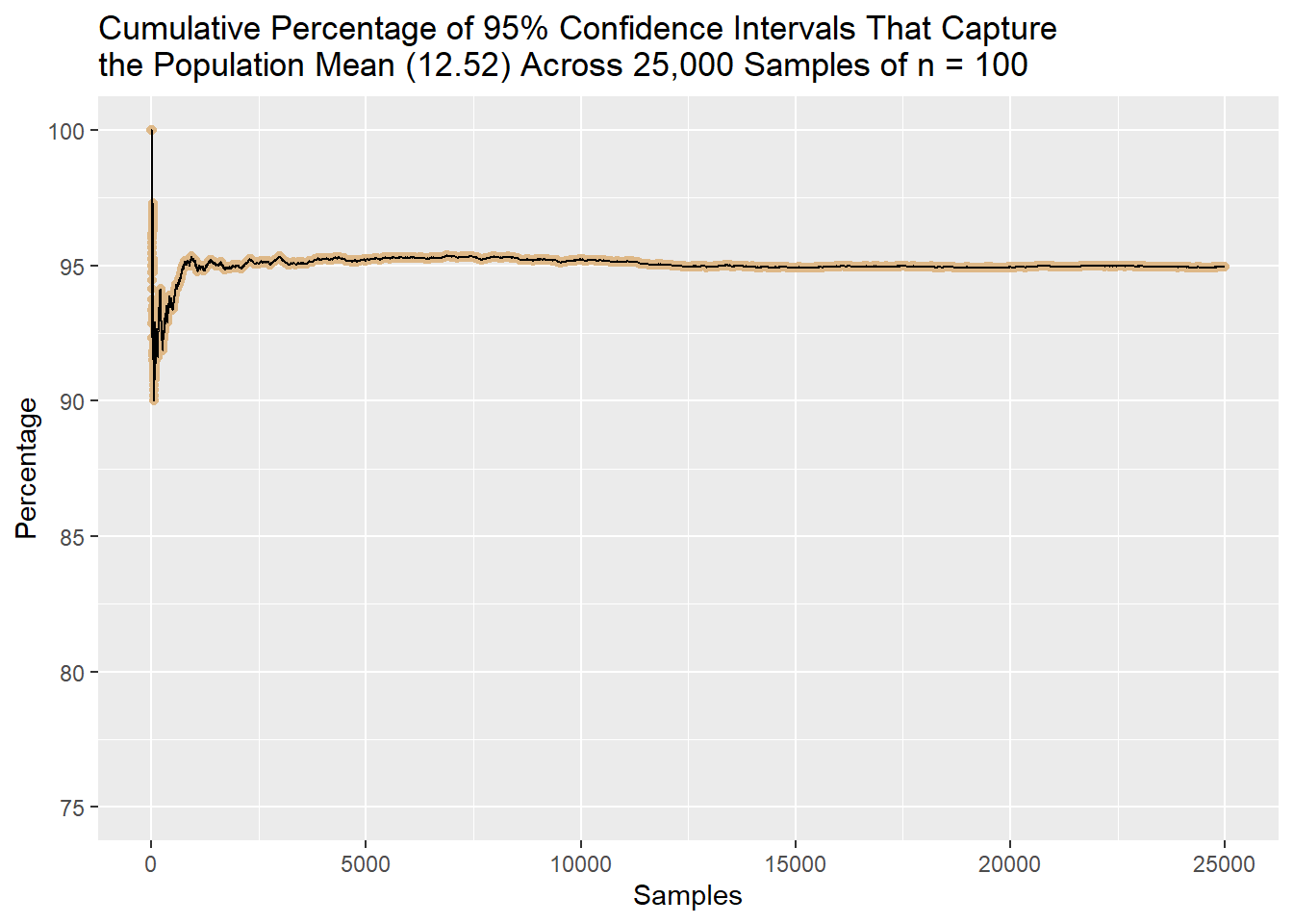
In this case, the confidence interval does capture the population mean (12.52). If I repeated the sampling and interval-calculation process over and over, the percentage of intervals that include 12.52 would converge to 95%. Below, I demonstrate exactly this: I draw 25,000 samples of \(n = 100\) from the population coffee data and calculate a 95% confidence interval around the sample mean each time. I then plot the cumulative percentage of intervals that capture the population mean across all 25,000 samples. The percentage drives toward and then stabilizes at 95%.


captures_true_mean <- vector(length = 25000)
for (i in 1:25000) {
  samp <- sample(coffee$grams, 100, replace = F)
  samp_se <- sd(samp) / sqrt(100)
  samp_radius <- samp_se * qt(0.975, df = 99)
  samp_lower <- mean(samp) - samp_radius
  samp_upper <- mean(samp) + samp_radius
  if (mean(coffee$grams) >= samp_lower & mean(coffee$grams) <= samp_upper) {
    captures_true_mean[i] <- 1} else {
      captures_true_mean[i] <- 0
    }
}

percentage_captures <- vector(length = 25000)
for (i in 1:length(captures_true_mean)) {
  percentage_captures[i] <- (sum(captures_true_mean[1:i]) / i)*100
}

ggplot(data.frame(perc = percentage_captures), aes(x = 1:length(perc), y = percentage_captures)) +
  geom_point(color = 'burlywood') + geom_line(color = 'black') + ylim(c(75, 100)) +
  labs(x = 'Samples', y = 'Percentage',
       title = paste0('Cumulative Percentage of 95% Confidence Intervals That Capture',
                      '\nthe Population Mean (12.52) Across 25,000 Samples of n = 100'))

cumulative proportion of 25,000 confidence intervals that capture the population parameter, converging to 95%

Jacob Goldstein-Greenwood
StatLab Associate
University of Virginia Library
October 25, 2021

A brief aside: \(n-1\) is commonly used instead of \(n\) alone when calculating the sample standard deviation, \(s\). That is:
\(s = \sqrt{\frac{1}{n-1}\sum_{i=1}^{n}(x_i - \bar{x})^2}\) instead of \(s = \sqrt{\frac{1}{n}\sum_{i=1}^{n}(x_i - \bar{x})^2}\)
This is Bessel’s correction; it’s an attempt to reduce bias when estimating the population standard deviation from the sample standard deviation. ↩︎
The reasoning behind using \(t_{0.975,\ n-1}^*\) instead of 1.96 to calculate a 95% confidence interval when the standard error is estimated using the sample standard deviation instead of the population standard deviation may not be immediately clear. I’ll try to briefly build the intuition here. Once we estimate the sampling distribution’s standard error, we need to determine how many standard errors out from the center of the sampling distribution we’d need to travel in both directions to capture 95% of the values therein. To sort this out, consider first how we arrive at 1.96 when the population standard deviation is known. Imagine that we were to take every sample mean in a sampling distribution and put each one in terms of the number of standard errors it lies from the center of the sampling distribution, with the standard error calculated using the population standard deviation. This is calculating a z statistic for every sample mean:
\(z = \frac{\bar{x} - \mu}{\frac{\sigma}{\sqrt{n}}}\)
A set of z statistics form a z distribution, which is normally distributed with a standard deviation of 1. We can consider how far out we’d need to travel in both directions from the center of the z distribution to capture 95% of its values (i.e., “What’s the 97.5% [or 2.5%] quantile of the z distribution?”): \(z_{0.975}^* = 1.96\). We know, then, that when the standard error is calculated using the population standard deviation, we would capture 95% of the points in the sampling distribution by traveling 1.96 standard errors out in each direction from the sampling distribution’s center:
\(J_{\sigma\ known} = 1.96 * SE\) (where \(SE = \frac{\sigma}{\sqrt{n}}\))
Imagine now that we don’t know the population standard deviation, and we instead were to put every sample mean in a sampling distribution in terms of the number of standard errors it lies from the center of the sampling distribution, with the standard error calculated using the sample standard deviation. This is calculating a t statistic for every sample mean:
\(t = \frac{\bar{x} - \mu}{\frac{s}{\sqrt{n}}}\)
A set of t statistics form a t distribution, which is similar but not equal to a normal distribution. The shape of the t distribution varies with n (whereas the shape of the z distribution does not). We can consider how far out we’d need to travel in both directions from the center of the t distribution to capture 95% of its values (i.e., “What’s the 97.5% [or 2.5%] quantile of the t distribution?”): \(t_{0.975,\ n-1}^*\). Each t statistic reflects a certain number of standard errors, where the standard error is calculated using the sample standard deviation. We know, then, that when the standard error is calculated using the sample standard deviation, we would capture 95% of the points in the sampling distribution by traveling \(t_{0.975,\ n-1}^*\) standard errors out in each direction from the sampling distribution’s center:
\(J_{\sigma\ unknown} = t_{0.975,\ n-1}^* * SE\) (where \(SE = \frac{s}{\sqrt{n}}\)) ↩︎

References

- R Core Team (2025). R: A Language and Environment for Statistical Computing. R Foundation for Statistical Computing, Vienna, Austria. https://www.R-project.org/.
- Wickham H (2016). ggplot2: Elegant Graphics for Data Analysis. Springer-Verlag, New York.