
From 2004 to 2008, a series of four brief, disagreeing papers in the journal Medical Education took up the question of whether and when it’s appropriate to analyze data from Likert scales (i.e., integers reflecting degrees of agreement with statements) with parametric or nonparametric statistical methods.
Although no overly convincing consensus emerged, at least in my view, the salvos fired brought up interesting considerations. For example, at the tail end of the exchange, Carifio and Perla (2008) distinguished between data from a single Likert item (ordered integers) and averages of data from two or more Likert items, arguing that the latter better approximate interval data and are well-suited to analysis with parametric tests.1 My aim here, however, isn’t to recapitulate the arc of the argument; my focus is on a premise that came up in the last three pieces in the exchange: That parametric tests are more powerful than nonparametric tests. That is, when some non-null finding is really there to be found, a parametric test is going to do a better job of “detecting” it than the test’s nonparametric sibling.
First, in a reply to the paper that sparked the exchange (Jamieson, 2004, which argued for analyzing Likert data with nonparametric methods), Pell (2005) said:
…[W]here there is an equivalent nonparametric test, it should be remembered that these are less powerful than the corresponding parametric test, so care should be exercised in drawing inference from any test statistics close to the critical value. (p. 970)
No caveat or condition appeared nearby to that language; the claim was made rather sweepingly. In a reply, Jamieson (2005) said:
Mr Pell also cautions that nonparametric tests are “less powerful” than the corresponding parametric tests (power being the ability to correctly reject the null hypothesis). However, Pett [1997] points out (p.26) that “a powerful test is also one whose assumptions have been sufficiently met.” She expands on this to say that serious departures from the underlying assumptions render a parametric test less powerful than the corresponding nonparametric test; and Sheskin [2000] acknowledges that “the power advantage of a parametric test may be negated if one or more of its assumptions are violated.” (p. 971)
Jamieson’s claim here is nuanced. She quotes work suggesting that when the assumptions of a parametric test break down (e.g., conditional normality, homogeneity of variance), its nonparametric alternative can be more powerful. But the underlying premise, communicated via the Pett and Sheskin quotes, is still that there is a “power advantage” of parametric tests in circumstances where their assumptions are not violated.
Finally, in the last paper of the exchange, Carifio and Perla (2008) said:
Nonparametric statistics, however, are less sensitive and less powerful than parametric statistics and are, therefore, more likely to miss weaker or emerging findings. (p. 1150)
This statement, like Pell’s (2005), was not accompanied by a nearby qualification; it’s a broad indictment of the power of nonparametric tests.
The “common denominator” position that Jamieson, Pell, and Carifio and Perla would seem to agree with (at least at the time their papers were written) is that under conditions in which the assumptions of a parametric test are satisfied, it will have some compelling power advantage over its nonparametric counterpart. Pell’s and Carifio and Perla’s statements also betray agreement with a whole lot more than just that limited view—the conditions, if any, under which they believe(d) that parametric tests wouldn’t edge out their counterparts aren’t described—but the minimal thread of agreement in the papers is an assertion of some meaningful power advantage of parametric tests under assumption-satisfying conditions.
This was worth investigating. I opted to compare the power of the parametric independent-samples t-test to its nonparametric sibling, the Mann-Whitney-Wilcoxon test. (The Mann-Whitney-Wilcoxon test is also called the Mann-Whitney U test and the Wilcoxon rank-sum test. For brevity, I call the test the “Wilcoxon test” hereafter, but it shouldn’t be confused with the Wilcoxon signed-rank test, which is a nonparametric test for evaluating paired differences.)
Power analysis by simulation was my comparative method of choice. (An article by my StatLab colleague Clay Ford on this method can be found here.) The conditions of the simulation were maximally conducive to the t-test’s assumptions, so as to assess the “common denominator” position that the Medical Education papers can be reasonably said to concur with.
I first wrote a function to estimate the power of the t-test and Wilcoxon test given a specified N, population-level mean difference between groups, and population-level standard deviation. The function makes a random draw of size N from each of two normal distributions given by \(\mathcal{N}(\mu_1, \sigma)\) and \(\mathcal{N}(\mu_2, \sigma)\). It then performs both a t-test and a Wilcoxon test comparing the two groups and saves the p-value from each. The process of drawing and testing is repeated a specified number of times, and power is taken as the fraction of p-values falling below .05.
t.wmw.pwr.sim <- function(n_per_grp = 100, grp1_mean = 3, grp2_mean = 3.5,
                          grp1_sd = 1, grp2_sd = 1, iters = 5000) {
  res <- replicate(iters, {
    x <- c(rep('a', n_per_grp), rep('b', n_per_grp))
    y <- c(rnorm(n_per_grp, grp1_mean, grp1_sd), rnorm(n_per_grp, grp2_mean, grp2_sd))
    t_res <- t.test(y ~ x, var.equal = T)
    wmw_res <- wilcox.test(y ~ x)
    list('t_pwr' = t_res$p.value, 'wmw_pwr' = wmw_res$p.value)
  }, simplify = T)
  res <- data.frame(t(res))
  c('t_pwr' = sum(res$t_pwr < .05) / iters, 'wmw_pwr' = sum(res$wmw_pwr < .05) / iters)
}
I then used the function to calculate the power of each test at a variety of per-group sample sizes (Ns = 25, 75, 175, and 250) and population-level mean differences. (The population standard deviations were fixed to one in all cases.)
# Simulation conditions
set.seed(2022)
mdiffs <- seq(0, .5, by = .05)
ns <- seq(25, 250, by = 75)
pwr_across_ns <- vector(mode = 'list', length = length(ns))
iters <- 5000

# Simulation
for (z in 1:length(ns)) {
  pwr <- data.frame(t_pwr = NA, wmw_pwr = NA, mdiff = mdiffs, n = ns[z])
  pwr[, c('t_pwr', 'wmw_pwr')] <- t(sapply(mdiffs, function(x) t.wmw.pwr.sim(n_per_grp = ns[z],
                                                                             grp1_mean = 3,
                                                                             grp2_mean = (3 + x),
                                                                             iters = iters)))
  pwr_across_ns[[z]] <- pwr
  if (z == length(ns)) {pwr <- data.table::rbindlist(pwr_across_ns)}
}
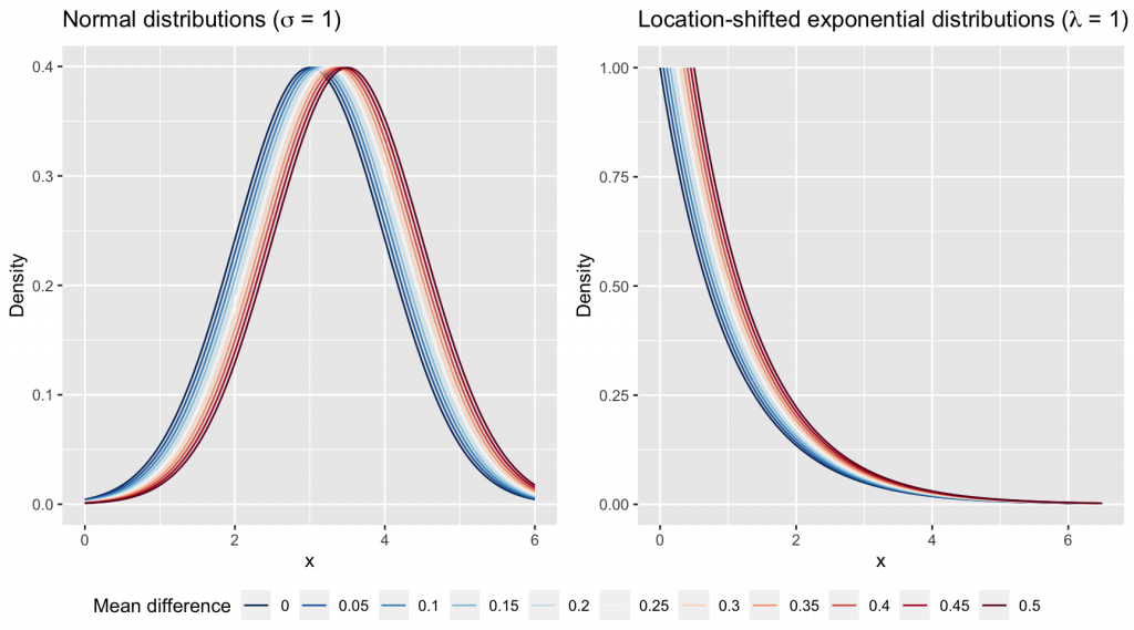
A plot of the results, faceted by per-group N, is below. (The distributions from which samples were drawn are visible in the plot following the references at the bottom of this piece.)
library(ggplot2)
library(tidyr)
long_pwr <- pivot_longer(pwr, cols = c(t_pwr, wmw_pwr), names_to = 'test', values_to = 'pwr')

ggplot(long_pwr, aes(x = mdiff, y = pwr, color = test)) +
  geom_point() + geom_line() +
  facet_wrap(~n, labeller = labeller(n = function(val) paste0('Per-group N = ', val))) +
  labs(title = expression(paste('Power comparison of ', italic(t), '-test and Wilcoxon test')),
       subtitle = expression(paste('Estimated by simulation: 5000 random samples taken from ',
                                   italic(N), '(', mu[1], ', ', 1, ')', ' and ',
                                   italic(N), '(', mu[2], ', ', 1, ')', ' underlie each point')),
       x = expression(atop('Mean difference',
                           paste(mu[1] == 3, "; ", mu[2] == 3, ' + Mean difference'))),
       y = 'Power') +
  scale_color_manual('Test type',
                     values = c('salmon', 'cornflowerblue'),
                     labels = c('t-test', 'Wilcoxon test')) +
  theme(legend.position = 'bottom')
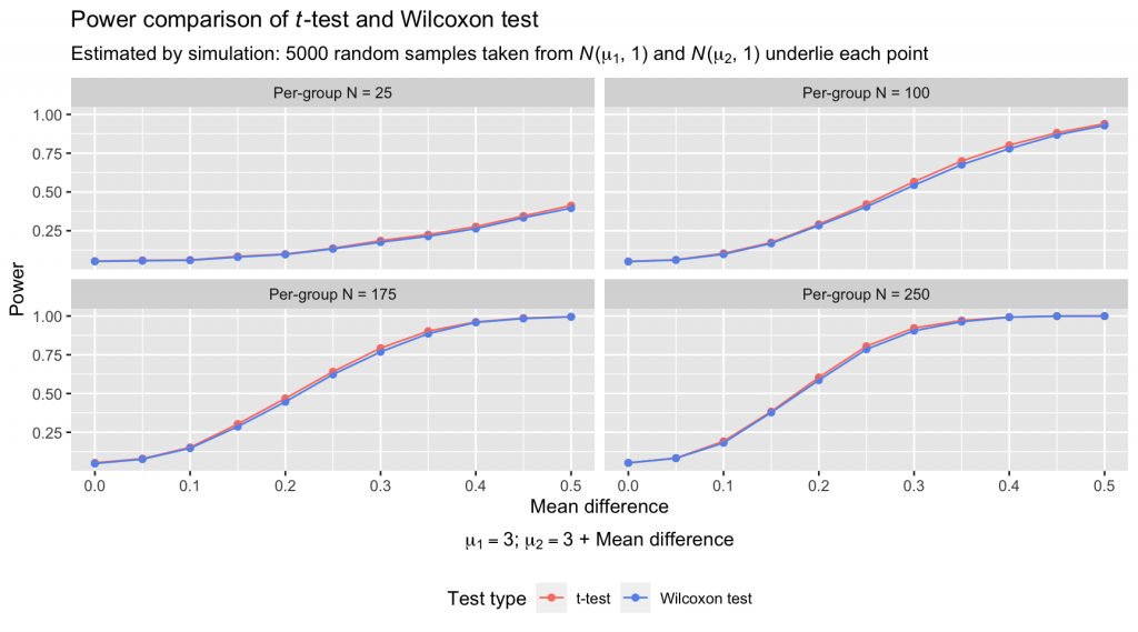
The power of the tests at each sample size and mean difference is nearly identical. Advantages of a percent or two are squeezed out here and there by the t-test, but I’d argue that there’s no difference in these plots worth losing sleep over. The average power difference between the t-test and Wilcoxon test across all pairs of points was a meager 0.0093, with a range of pairwise differences of [-0.0002, 0.0240]. Essential to remember is that the data simulation was designed to be maximally conducive to the t-test’s performance: Samples were drawn from normal distributions with identical variances. These conditions are often violated in real data sets, which tempers my faith that the small power advantages of the t-test observed above are realized with much frequency.
We have here a case of similar power, even under conditions optimized for the parametric test. Beyond simply keeping pace with the t-test in the case above, the Wilcoxon test outperforms the t-test in many circumstances in which the latter’s assumptions are ill-met. Below, I repeat the simulation from above but now draw samples from exponential distributions with rates (\(\lambda\)) of 1, and I add a constant to the values in one group on each iteration to induce a mean difference between the groups. (The distributions sampled from in this simulation are shown in the plot at the bottom of this article.)
t.wmw.pwr.sim.exp <- function(n_per_grp = 100, rate = 1, mdiff = .25, iters = 5000) {
  res <- replicate(iters, {
    x <- c(rep('a', n_per_grp), rep('b', n_per_grp))
    y <- c(rexp(n_per_grp, rate), (rexp(n_per_grp, rate) + mdiff))
    t_res <- t.test(y ~ x, var.equal = T)
    wmw_res <- wilcox.test(y ~ x)
    list('t_pwr' = t_res$p.value, 'wmw_pwr' = wmw_res$p.value)
  }, simplify = T)
  res <- data.frame(t(res))
  c('t_pwr' = sum(res$t_pwr < .05) / iters, 'wmw_pwr' = sum(res$wmw_pwr < .05) / iters)
}

# Simulation conditions
set.seed(2022)
mdiffs <- seq(0, .5, by = .05)
ns <- seq(25, 250, by = 75)
pwr_across_ns <- vector(mode = 'list', length = length(ns))
iters <- 5000

# Simulation
for (z in 1:length(ns)) {
  pwr <- data.frame(t_pwr = NA, wmw_pwr = NA, mdiff = mdiffs, n = ns[z])
  pwr[, c('t_pwr', 'wmw_pwr')] <- t(sapply(mdiffs, function(x) t.wmw.pwr.sim.exp(n_per_grp = ns[z],
                                                                                 rate = 1,
                                                                                 mdiff = x,
                                                                                 iters = iters)))
  pwr_across_ns[[z]] <- pwr
  if (z == length(ns)) {pwr <- data.table::rbindlist(pwr_across_ns)}
}

long_pwr <- pivot_longer(pwr, cols = c(t_pwr, wmw_pwr), names_to = 'test', values_to = 'pwr')

ggplot(long_pwr, aes(x = mdiff, y = pwr, color = test)) +
  geom_point() + geom_line() +
  facet_wrap(~n, labeller = labeller(n = function(val) paste0('Per-group N = ', val))) +
  labs(title = expression(paste('Power comparison of ', italic(t), '-test and Wilcoxon test')),
       subtitle = expression(paste('Estimated by simulation: 5000 random samples taken from ',
                                   'exponential distributions with rate (',
                                   lambda, ') = 1 underlie each point')),
       x = expression(atop('Mean difference',
                           paste(mu[1] == 1, "; ", mu[2] == 1, ' + Mean difference'))),
       y = 'Power') +
  scale_color_manual('Test type',
                     values = c('salmon', 'cornflowerblue'),
                     labels = c('t-test', 'Wilcoxon test')) +
  theme(legend.position = 'bottom')
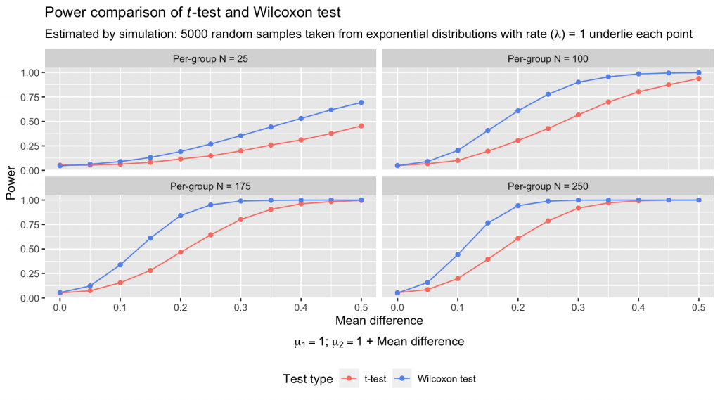
The power of the Wilcoxon test far exceeds that of the t-test under these conditions, with an average pairwise power advantage of 0.1407 and a maximum advantage of 0.3754. And these kinds of skewed distributions are far from unrealistic: Many kinds of values that an analyst might have reflexively compared with a t-test are distributed with such asymmetric, stretching tails.
These simulations suggest that the assertions of a wholesale power advantage for parametric tests made by Pell (2005) and Carifio and Perla (2008) can’t be sustained. Finding a case in which a parametric test’s power collapses compared to its nonparametric counterpart isn’t difficult. Even Jamieson’s (2005) more-nuanced position—that parametric tests hold power advantages when their assumptions are satisfied—has to be interpreted carefully: The power advantages that the t-test sometimes squeezed out under optimized conditions in the simulation above were minute—certainly not large enough to take as evidence of radical superiority when its assumptions are satisfied. And real data sets often violate those assumptions.
These results aren’t surprising. Many analysts and researchers have performed similar simulations comparing the power of parametric and nonparametric tests, covering a range of scenarios beyond the cases considered here. In a thoroughly readable 1980 paper in the Journal of Educational Statistics, Blair and Higgins compared the power of the t-test and Wilcoxon test when sampling from uniform, Laplace, half-normal, exponential, mixed-normal, and mixed-uniform distributions. For per-group sample sizes of 36 and 108 (“moderate” Ns in their parlance), they observed that under the uniform distribution, the t-test had a hair more power, but the Wilcoxon test dominated in the other five cases. A central part of their takeaway is that while the t-test achieves modest power advantages under some conditions, that superiority is never particularly large, whereas the Wilcoxon test achieves sizable and consistent power advantages in many cases in which the t-test’s assumptions are not satisfied.
Power is by no means the sole metric by which to compare tests; one can just as seriously consider the circumstances under which parametric and nonparametric methods maintain their nominal Type I error rates. Differences in the specific hypotheses being tested are also relevant: The null hypothesis of the two-sample t-test is that the means of two groups are equal (with the alternative hypothesis being that the means differ); the null hypothesis of the Wilcoxon test is that the probability distributions of two groups are equal (with the alternative hypothesis being that the values in one group tend to be larger than the values in the other; Hollander, Wolfe, & Chicken, 2013). Both tests attack the question of which of two groups has generally larger values (Fay & Proschan, 2010), but the result of one shouldn’t be framed as though it communicates an identical conclusion as the other. The t-test has broad applications and impressive robustness to assumption violations, but the notion that it and other parametric tests enjoy a sweeping, no-caveats-needed power advantage over nonparametric tests isn’t justified.
R session details
The analysis was done using the R Statistical language (v4.5.2; R Core Team, 2025) on Windows 11 x64, using the packages ggplot2 (v4.0.1) and tidyr (v1.3.1).
References
- Blair, R. C., & Higgins, J. J. (1980). A comparison of the power of Wilcoxon’s rank-sum statistic to that of Student’s t statistic under various nonnormal distributions. Journal of Educational Statistics, 5(4), 309–335. https://doi.org/10.3102/10769986005004309
- Carifio, J., & Perla, R. (2008). Resolving the 50-year debate around using and misusing Likert scales. Medical Education, 42(12), 1150–1152. https://onlinelibrary.wiley.com/doi/10.1111/j.1365-2923.2008.03172.x
- Fay, M. P., & Proschan, M. A. (2010). Wilcoxon-Mann-Whitney or t-test? On assumptions for hypothesis tests and multiple interpretations of decision rules. Statistics Surveys, 4, 1–39. https://doi.org/10.1214/09-SS051
- Hollander, M., Wolfe, D. A., & Chicken, E. (2013). Nonparametric statistical methods (3rd ed.). John Wiley & Sons.
- Jamieson, S. (2004). Likert scales: How to (ab)use them? Medical Education, 38(12), 1217–1218. https://doi.org/10.1111/j.1365-2929.2004.02012.x
- Jamieson, S. (2005). Author’s reply. Medical Education, 39(9), 971. https://onlinelibrary.wiley.com/doi/10.1111/j.1365-2929.2005.02238.x
- Pell, G. (2005). Use and misuse of Likert scales. Medical Education, 39(9), 970. https://onlinelibrary.wiley.com/doi/10.1111/j.1365-2929.2005.02237.x
Distributions from which samples were drawn for each simulation
# Normal distributions
domain <- seq(0, 6, by = .01)
plt_dat <- data.frame(mapply(dnorm, rep(list(domain), times = length(mdiffs)), 3 + mdiffs, 1))
colnames(plt_dat) <- mdiffs
plt_dat$x <- domain
plt_dat <- tidyr::pivot_longer(plt_dat, cols = -x, names_to = 'mdiff', values_to = 'y')
normal_plts <- ggplot(plt_dat, aes(x = x, y = y, color = mdiff)) +
  geom_line() +
  labs(title = expression(paste('Normal distributions (',
                                sigma, ' = 1)')), y = 'Density') +
  scale_color_brewer('Mean difference', palette = 'RdBu', direction = -1) +
  guides(color = guide_legend(nrow = 1))

# Location-shifted exponential distributions
domain <- seq(0, 6, by = .01)
y <- dexp(domain, rate = 1)
plt_dat <- data.frame(domain = domain, y = y, mdiff = 0)
for (i in 2:length(mdiffs)) {
  tmp <- data.frame(domain = domain + mdiffs[i], y = y, mdiff = as.character(mdiffs[i]))
  plt_dat <- rbind(plt_dat, tmp)
}
exp_plts <- ggplot(plt_dat, aes(x = domain, y = y, color = mdiff)) +
  geom_line() +
  labs(title = expression(paste('Location-shifted exponential distributions (',
                                lambda, ' = 1)')), x = 'x', y = 'Density') +
  scale_color_brewer('Mean difference', palette = 'RdBu', direction = -1) +
  guides(color = guide_legend(nrow = 1))

ggpubr::ggarrange(normal_plts, exp_plts, nrow = 1, common.legend = T, legend = 'bottom')
Jacob Goldstein-Greenwood
Research Data Scientist
University of Virginia Library
October 28, 2022
- Carifio and Perla (2008) didn’t make this point, but I note for the curious: Respondent-level averages on a k-item Likert scale in which items are scored as integers ranging from x to y must have decimal parts that are multiples of \(\frac{1}{k}\). Any given respondent’s average on the k items must be \(z + (j*\frac{1}{k})\), where \(z \in [x..(y-1)]\) and \(j \in [0..k]\). As k increases, the granularity of the respondent-level averages can increase. ↩︎
For questions or clarifications regarding this article, contact statlab@virginia.edu.
View the entire collection of UVA Library StatLab articles, or learn how to cite.