Is R-squared Useless?

On Thursday, October 15, 2015, a disbelieving student posted on Reddit: My stats professor just went on a rant about how R-squared values are essentially useless, is there any truth to this? It attracted a fair amount of attention, at least compared to other posts about statistics on Reddit.

It turns out the student's stats professor was Cosma Shalizi of Carnegie Mellon University. Shalizi provides free and open access to his class lecture materials, so we can see what exactly he was "ranting" about. It all begins in Section 3.2 of his Lecture 10 notes.

In case you forgot or didn't know, R-squared is a statistic that often accompanies regression output. It ranges in value from 0 to 1 and is usually interpreted as summarizing the percent of variation in the response that the regression model explains. So an R-squared of 0.65 might mean that the model explains about 65% of the variation in our dependent variable. Given this logic, we prefer our regression models to have a high R-squared. Shalizi, however, disputes this logic with convincing arguments.

In R, we typically get R-squared by calling the summary function on a model object. Here's a quick example using simulated data:

x <- 1:20                        # independent variable
set.seed(1)                      # for reproducibility
y <- 2 + 0.5*x + rnorm(20,0,3)   # dependent variable; function of x with random error
mod <- lm(y~x)                   # simple linear regression
summary(mod)$r.squared           # request just the r-squared value

[1] 0.6026682

One way to express R-squared is as the sum of squared fitted-value deviations divided by the sum of squared original-value deviations: $$R^{2} = \frac{\sum (\hat{y} - \bar{\hat{y}})^{2}}{\sum (y - \bar{y})^{2}} $$ We can calculate it directly using our model object like so:

f <- mod$fitted.values       # extract fitted (or predicted) values from model
mss <- sum((f - mean(f))^2)  # sum of squared fitted-value deviations
tss <- sum((y - mean(y))^2)  # sum of squared original-value deviations
mss/tss                      # r-squared

[1] 0.6026682

Now let's take a look at a few of Shalizi's statements about R-squared and demonstrate them with simulations in R.

1. R-squared does not measure goodness of fit. It can be arbitrarily low when the model is completely correct. By making \(\sigma^{2}\) large, we drive R-squared towards 0, even when every assumption of the simple linear regression model is correct in every particular.

What is \(\sigma^{2}\)? When we perform linear regression, we assume our model almost predicts our dependent variable. The difference between "almost" and "exact" is assumed to be a draw from a normal distribution with mean 0 and some variance we call \(\sigma^{2}\).

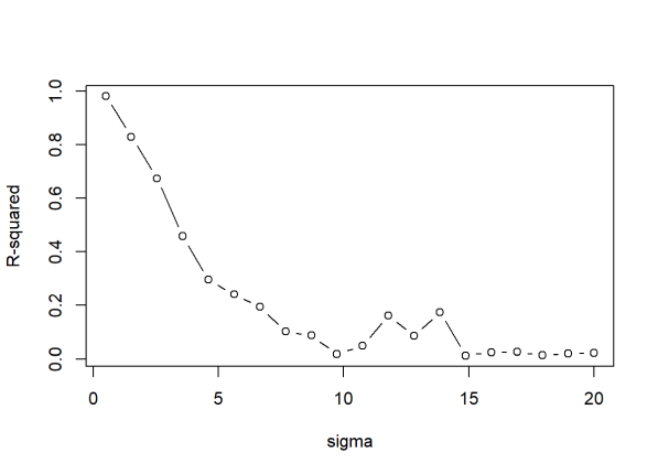
Shalizi's statement is easy enough to demonstrate. The way we do it here is to create a function that (1) generates data meeting the assumptions of simple linear regression (independent observations, normally distributed errors with constant variance), (2) fits a simple linear model to the data, and (3) reports the R-squared. Notice the only parameter for sake of simplicity is sig (sigma). We then "apply" this function to a series of increasing \(\sigma\) values and plot the results.

r2.0 <- function(sig){
  x <- seq(1,10,length.out = 100)        # our predictor
  y <- 2 + 1.2*x + rnorm(100,0,sd = sig) # our response; a function of x plus some random noise
  summary(lm(y ~ x))$r.squared           # print the R-squared value
}

sigmas <- seq(0.5,20,length.out = 20)
rout <- sapply(sigmas, r2.0)             # apply our function to a series of sigma values
plot(rout ~ sigmas, type="b")

Sure enough, R-squared tanks hard with increasing sigma, even though the model is completely correct in every respect.

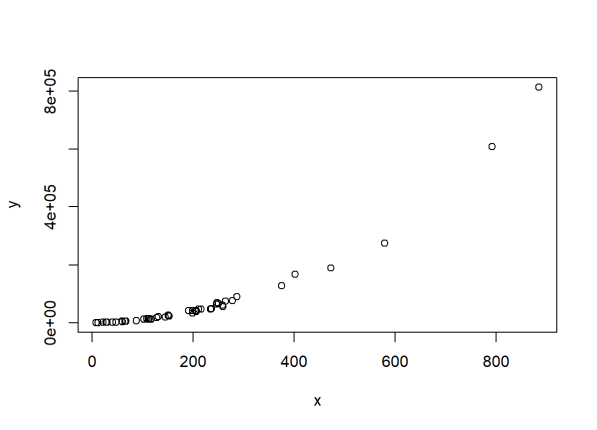
2. R-squared can be arbitrarily close to 1 when the model is totally wrong. Again, the point being made is that R-squared does not measure goodness of fit. Here we use code from a different section of Shalizi's lecture 10 notes to generate non-linear data.

set.seed(1)
x <- rexp(50,rate=0.005)                     # our predictor is data from an exponential distribution
y <- (x-1)^2 * runif(50, min=0.8, max=1.2)   # non-linear data generation
plot(x,y)				     # clearly non-linear

Now check the R-squared:

summary(lm(y ~ x))$r.squared

[1] 0.8485146

It's very high at about 0.85, but the model is completely wrong. Using R-squared to justify the "goodness" of our model in this instance would be a mistake. Hopefully one would plot the data first and recognize that a simple linear regression in this case would be inappropriate.

3. R-squared says nothing about prediction error, even with \(\sigma^{2}\) exactly the same, and no change in the coefficients. R-squared can be anywhere between 0 and 1 just by changing the range of X. We're better off using Mean Square Error (MSE) as a measure of prediction error.

MSE is basically the fitted y values minus the observed y values, squared, then summed, and then divided by the number of observations.

Let's demonstrate this statement by first generating data that meets all simple linear regression assumptions and then regressing y on x to assess both R-squared and MSE.

x <- seq(1,10,length.out = 100)
set.seed(1)
y <- 2 + 1.2*x + rnorm(100,0,sd = 0.9)
mod1 <- lm(y ~ x)
summary(mod1)$r.squared

[1] 0.9383379

sum((fitted(mod1) - y)^2)/100 # Mean squared error

[1] 0.6468052

Now repeat the above code, but this time with a different range of x. Leave everything else the same:

x <- seq(1,2,length.out = 100)       # new range of x
set.seed(1)
y <- 2 + 1.2*x + rnorm(100,0,sd = 0.9)
mod1 <- lm(y ~ x)
summary(mod1)$r.squared

[1] 0.1502448

sum((fitted(mod1) - y)^2)/100        # Mean squared error

[1] 0.6468052

The R-squared falls from 0.94 to 0.15 but the MSE remains the same. In other words the predictive ability is the same for both data sets, but the R-squared would lead you to believe the first example somehow had a model with more predictive power.

4. R-squared cannot be compared between a model with untransformed Y and one with transformed Y, or between different transformations of Y. R-squared can easily go down when the model assumptions are better fulfilled.

Let's examine this by generating data that would benefit from transformation. Notice the R code below is very much like our previous efforts but now we exponentiate our y variable.

x <- seq(1,2,length.out = 100)
set.seed(1)
y <- exp(-2 - 0.09*x + rnorm(100,0,sd = 2.5))
summary(lm(y ~ x))$r.squared

[1] 0.003281718

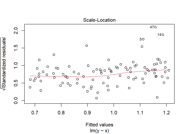
plot(lm(y ~ x), which=3)

R-squared is very low and our residuals vs. fitted plot reveals outliers and non-constant variance. A common fix for this is to log transform the data. Let's try that and see what happens:

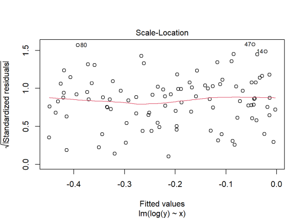
plot(lm(log(y)~x),which = 3) 

The diagnostic plot looks much better. Our assumption of constant variance appears to be met. But look at the R-squared:

summary(lm(log(y)~x))$r.squared

[1] 0.0006921086

It's even lower! This is an extreme case and it doesn't always happen like this. In fact, a log transformation will usually produce an increase in R-squared. But as just demonstrated, assumptions that are better fulfilled don't always lead to higher R-squared. And hence R-squared cannot be compared between models with different transformations of the outcome.

5. It is very common to say that R-squared is "the fraction of variance explained" by the regression. [Yet] if we regressed X on Y, we'd get exactly the same R-squared. This in itself should be enough to show that a high R-squared says nothing about explaining one variable by another. This is the easiest statement to demonstrate:

x <- seq(1,10,length.out = 100)
y <- 2 + 1.2*x + rnorm(100,0,sd = 2)
summary(lm(y ~ x))$r.squared

[1] 0.7065779

summary(lm(x ~ y))$r.squared

[1] 0.7065779

Does x explain y, or does y explain x? Are we saying "explain" to dance around the word "cause"? In a simple scenario with two variables such as this, R-squared is simply the square of the correlation between x and y:

all.equal(cor(x,y)^2, summary(lm(x ~ y))$r.squared, summary(lm(y ~ x))$r.squared)

[1] TRUE

Why not just use correlation instead of R-squared in this case? But then again correlation summarizes linear relationships, which may not be appropriate for the data. This is another instance where plotting your data is strongly advised. Let's recap:

• R-squared does not measure goodness of fit.
• R-squared does not measure predictive error.
• R-squared does not allow you to compare models using transformed responses.
• R-squared does not measure how one variable explains another.

And that's just what we covered in this article. Shalizi gives even more reasons in his lecture notes. And it should be noted that adjusted R-squared does nothing to address any of these issues. So is there any reason at all to use R-squared? Shalizi says no. ("I have never found a situation where it helped at all.") No doubt, some statisticians and Redditors might disagree. Whatever your view, if you choose to use R-squared to inform your data analysis, it would be wise to double-check that it's telling you what you think it's telling you.

Clay Ford
Statistical Research Consultant
University of Virginia Library
Oct 17, 2015

References

- R Core Team (2025). R: A Language and Environment for Statistical Computing. R Foundation for Statistical Computing, Vienna, Austria. https://www.R-project.org/.
- Shalizi, C. (2015). 36-401, Modern Regression, Section B [Course syllabus]. Carnegie Mellon University, Department of Statistics. https://www.stat.cmu.edu/~cshalizi/mreg/15/