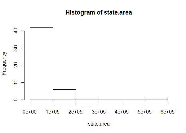
Log transformations are often recommended for skewed data, such as monetary measures or certain biological and demographic measures. Log transforming data usually has the effect of spreading out clumps of data and bringing together spread-out data. For example, below is a histogram of the areas of all 50 US states. It is skewed to the right due to Alaska, California, Texas and a few others.
hist(state.area)
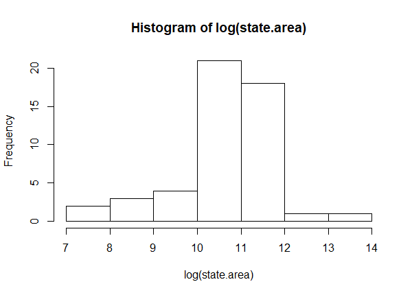
After a log transformation, notice the histogram is more or less symmetric. We've moved the big states closer together and spaced out the smaller states.
hist(log(state.area))
Why do this? One reason is to make data more "normal", or symmetric. If we're performing a statistical analysis that assumes normality, a log transformation might help us meet this assumption. Another reason is to help meet the assumption of constant variance in the context of linear modeling. Yet another is to help make a non-linear relationship more linear. But while it's easy to implement a log transformation, it can complicate interpretation. Let's say we fit a linear model with a log-transformed dependent variable. How do we interpret the coefficients? What if we have log-transformed dependent and independent variables? That's the topic of this article. First we'll provide a recipe for interpretation for those who just want some quick help. Then we'll dig a little deeper into what we're saying about our model when we log-transform our data.
Rules for interpretation
OK, you ran a regression/fit a linear model and some of your variables are log-transformed.
- Only the dependent/response variable is log-transformed. Exponentiate the coefficient. This gives the multiplicative factor for every one-unit increase in the independent variable. Example: the coefficient is 0.198. exp(0.198) = 1.218962. For every one-unit increase in the independent variable, our dependent variable increases by a factor of about 1.22, or 22%. Recall that multiplying a number by 1.22 is the same as increasing the number by 22%. Likewise, multiplying a number by, say 0.84, is the same as decreasing the number by 1 – 0.84 = 0.16, or 16%.
- Only independent/predictor variable(s) is log-transformed. Divide the coefficient by 100. This tells us that a 1% increase in the independent variable increases (or decreases) the dependent variable by (coefficient/100) units. Example: the coefficient is 0.198. 0.198/100 = 0.00198. For every 1% increase in the independent variable, our dependent variable increases by about 0.002. For x percent increase, multiply the coefficient by log(1.x). Example: For every 10% increase in the independent variable, our dependent variable increases by about 0.198 * log(1.10) = 0.02.
- Both dependent/response variable and independent/predictor variable(s) are log-transformed. Interpret the coefficient as the percent increase in the dependent variable for every 1% increase in the independent variable. Example: the coefficient is 0.198. For every 1% increase in the independent variable, our dependent variable increases by about 0.20%. For x percent increase, calculate 1.x to the power of the coefficient, subtract 1, and multiply by 100. Example: For every 20% increase in the independent variable, our dependent variable increases by about (1.20 0.198 - 1) * 100 = 3.7 percent.
What Log Transformations Really Mean for your Models
It's nice to know how to correctly interpret coefficients for log-transformed data, but it's important to know what exactly your model is implying when it includes log-transformed data. To get a better understanding, let's use R to simulate some data that will require log-transformations for a correct analysis. We'll keep it simple with one independent variable and normally distributed errors. First we'll look at a log-transformed dependent variable.
x <- seq(0.1,5,length.out = 100)
set.seed(1)
e <- rnorm(100, mean = 0, sd = 0.2)
The first line generates a sequence of 100 values from 0.1 to 5 and assigns it to x. The next line sets the random number generator seed to 1. If you do the same, you'll get the same randomly generated data that we got when you run the next line. The code rnorm(100, mean = 0, sd = 0.2) generates 100 values from a Normal distribution with a mean of 0 and standard deviation of 0.2. This will be our "error". This is one of the assumptions of simple linear regression: our data can be modeled with a straight line but will be off by some random amount that we assume comes from a Normal distribution with mean 0 and some standard deviation. We assign our error to e.
Now we're ready to create our log-transformed dependent variable. We pick an intercept (1.2) and a slope (0.2), which we multiply by x, and then add our random error, e. Finally we exponentiate.
y <- exp(1.2 + 0.2 * x + e)
To see why we exponentiate, notice the following: $$\text{log}(y) = \beta_0 + \beta_1x$$ $$\text{exp}(\text{log}(y)) = \text{exp}(\beta_0 + \beta_1x)$$ $$y = \text{exp}(\beta_0 + \beta_1x)$$ So a log-transformed dependent variable implies our simple linear model has been exponentiated. Recall from the product rule of exponents that we can re-write the last line above as $$y = \text{exp}(\beta_0) \text{exp}(\beta_1x)$$ This further implies that our independent variable has a multiplicative relationship with our dependent variable instead of the usual additive relationship. Hence the need to express the effect of a one-unit change in x on y as a percent.
If we fit the correct model to the data, notice we do a pretty good job of recovering the true parameter values that we used to generate the data.
lm1 <- lm(log(y) ~ x)
summary(lm1)
Call:
lm(formula = log(y) ~ x)

Residuals:
    Min      1Q  Median      3Q     Max
-0.4680 -0.1212  0.0031  0.1170  0.4595

Coefficients:
            Estimate Std. Error t value Pr(>|t|)
(Intercept)  1.22643    0.03693   33.20   <2e-16 ***
x            0.19818    0.01264   15.68   <2e-16 ***
---
Signif. codes:  0 ‘***’ 0.001 ‘**’ 0.01 ‘*’ 0.05 ‘.’ 0.1 ‘ ’ 1

Residual standard error: 0.1805 on 98 degrees of freedom
Multiple R-squared:  0.7151,	Adjusted R-squared:  0.7122
F-statistic:   246 on 1 and 98 DF,  p-value: < 2.2e-16
The estimated intercept of 1.226 is close to the true value of 1.2. The estimated slope of 0.198 is very close to the true value of 0.2. Finally the estimated residual standard error of 0.1805 is not too far from the true value of 0.2.
Recall that to interpret the slope value we need to exponentiate it.
exp(coef(lm1)["x"])
       x
1.219179
This says every one-unit increase in x is multiplied by about 1.22. Or in other words, for every one-unit increase in x, y increases by about 22%. To get 22%, subtract 1 and multiply by 100.
(exp(coef(lm1)["x"]) - 1) * 100
       x
21.91786
What if we fit just y instead of log(y)? How might we figure out that we should consider a log transformation? Just looking at the coefficients isn't going to tell you much.
lm2 <- lm(y ~ x)
summary(lm2)
Call:
lm(formula = y ~ x)

Residuals:
    Min      1Q  Median      3Q     Max
-2.3868 -0.6886 -0.1060  0.5298  3.3383

Coefficients:
            Estimate Std. Error t value Pr(>|t|)
(Intercept)  3.00947    0.23643   12.73   <2e-16 ***
x            1.16277    0.08089   14.38   <2e-16 ***
---
Signif. codes:  0 ‘***’ 0.001 ‘**’ 0.01 ‘*’ 0.05 ‘.’ 0.1 ‘ ’ 1

Residual standard error: 1.156 on 98 degrees of freedom
Multiple R-squared:  0.6783,	Adjusted R-squared:  0.675
F-statistic: 206.6 on 1 and 98 DF,  p-value: < 2.2e-16
Sure, since we generated the data, we can see the coefficients are way off and the residual standard error is much too high. But in real life you won't know this! This is why we do regression diagnostics. A key assumption to check is constant variance of the errors. We can do this with a Scale-Location plot. Here's the plot for the model we just ran without log transforming y.
plot(lm2, which = 3) # 3 = Scale-Location plot
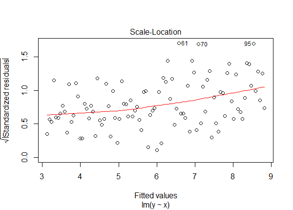
Notice the standardized residuals are trending upward. This is a sign that the constant variance assumption has been violated. Compare this plot to the same plot for the correct model.
plot(lm1, which = 3)
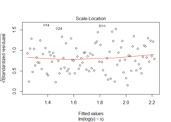
The trend line is even and the residuals are uniformly scattered.
Does this mean that you should always log-transform your dependent variable if you suspect the constant-variance assumption has been violated? Not necessarily. The non-constant variance may be due to other misspecifications in your model. Also think about what modeling a log-transformed dependent variable means. It says it has a multiplicative relationship with the predictors. Does that seem right? Use your judgment and subject expertise.
Now let's consider data with a log-transformed independent predictor variable. This is easier to generate. We simply log-transform x.
y <- 1.2 + 0.2*log(x) + e
Once again we first fit the correct model and notice it does a great job of recovering the true values we used to generate the data:
lm3 <- lm(y ~ log(x))
summary(lm3)
Call:
lm(formula = y ~ log(x))

Residuals:
     Min       1Q   Median       3Q      Max
-0.46492 -0.12063  0.00112  0.11661  0.45864

Coefficients:
            Estimate Std. Error t value Pr(>|t|)
(Intercept)  1.22192    0.02308  52.938  < 2e-16 ***
log(x)       0.19979    0.02119   9.427 2.12e-15 ***
---
Signif. codes:  0 ‘***’ 0.001 ‘**’ 0.01 ‘*’ 0.05 ‘.’ 0.1 ‘ ’ 1

Residual standard error: 0.1806 on 98 degrees of freedom
Multiple R-squared:  0.4756,	Adjusted R-squared:  0.4702
F-statistic: 88.87 on 1 and 98 DF,  p-value: 2.121e-15
To interpret the slope coefficient we divide it by 100.
coef(lm3)["log(x)"]/100
     log(x)
0.001997892
This tells us that a 1% increase in x increases the dependent variable by about 0.002. Why does it tell us this? Let's do some math. Below we calculate the change in y when changing x from 1 to 1.01 (ie, a 1% increase). $$(\beta_0 + \beta_1\text{log}1.01) - (\beta_0 + \beta_1\text{log}1)$$ $$\beta_1\text{log}1.01 - \beta_1\text{log}1$$ $$\beta_1(\text{log}1.01 - \text{log}1)$$ $$\beta_1\text{log}\frac{1.01}{1} = \beta_1\text{log}1.01$$ The result is multiplying the slope coefficient by log(1.01), which is approximately equal to 0.01, or \(\frac{1}{100}\). Hence the interpretation that a 1% increase in x increases the dependent variable by the coefficient/100.
Once again let's fit the wrong model by failing to specify a log-transformation for x in the model syntax.
lm4 <- lm(y ~ x)
Viewing a summary of the model will reveal that the estimates of the coefficients are well off from the true values. But in practice we never know the true values. Once again diagnostics are in order to assess model adequacy. A useful diagnostic in this case is a partial-residual plot which can reveal departures from linearity. Recall that linear models assume that predictors are additive and have a linear relationship with the response variable. The car package provides the crPlot() function for quickly creating partial-residual plots. Just give it the model object and specify which variable you want to create the partial residual plot for.
library(car)
crPlot(lm4, variable = "x")
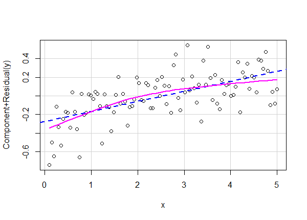
The straight line represents the specified relationship between x and y. The curved line is a smooth trend line that summarizes the observed relationship between x and y. We can tell the observed relationship is non-linear. Compare this plot to the partial-residual plot for the correct model.
crPlot(lm3, variable = "log(x)")
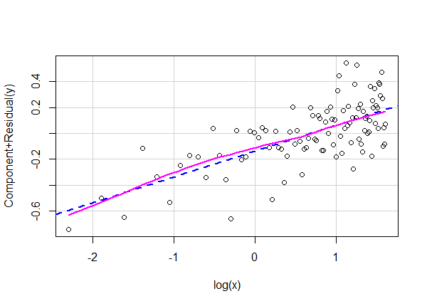
The smooth and fitted lines are right on top of one another revealing no serious departures from linearity.
This does not mean that if you see departures from linearity you should immediately assume a log transformation is the one and only fix! The non-linear relationship may be complex and not so easily explained with a simple transformation. But a log transformation may be suitable in such cases and certainly something to consider.
Finally let's consider data where both the dependent and independent variables are log transformed.
y <- exp(1.2 + 0.2 * log(x) + e)
Look closely at the code above. The relationship between x and y is now both multiplicative and non-linear!
As usual we can fit the correct model and notice that it does a fantastic job of recovering the true values we used to generate the data:
lm5 <- lm(log(y)~ log(x))
summary(lm5)
Call:
lm(formula = log(y) ~ log(x))

Residuals:
     Min       1Q   Median       3Q      Max
-0.46492 -0.12063  0.00112  0.11661  0.45864

Coefficients:
            Estimate Std. Error t value Pr(>|t|)
(Intercept)  1.22192    0.02308  52.938  < 2e-16 ***
log(x)       0.19979    0.02119   9.427 2.12e-15 ***
---
Signif. codes:  0 ‘***’ 0.001 ‘**’ 0.01 ‘*’ 0.05 ‘.’ 0.1 ‘ ’ 1

Residual standard error: 0.1806 on 98 degrees of freedom
Multiple R-squared:  0.4756,	Adjusted R-squared:  0.4702
F-statistic: 88.87 on 1 and 98 DF,  p-value: 2.121e-15
Interpret the x coefficient as the percent increase in y for every 1% increase in x. In this case that's about a 0.2% increase in y for every 1% increase in x.
Fitting the wrong model once again produces coefficient and residual standard error estimates that are wildly off target.
lm6 <- lm(y ~ x)
summary(lm6)
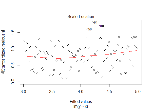
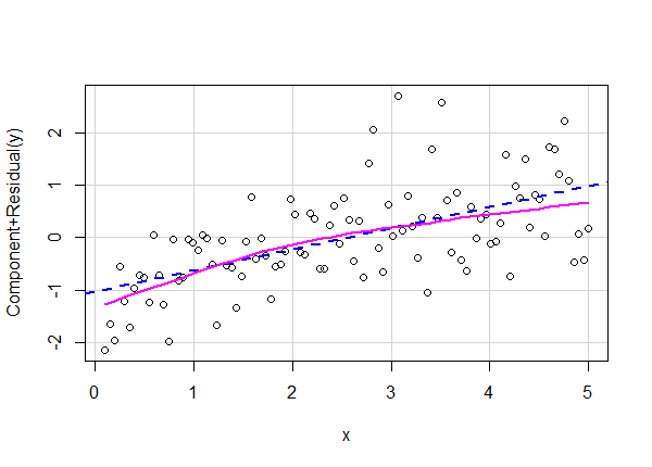
The Scale-Location and Partial-Residual plots provide evidence that something is amiss with our model. The Scale-Location plot shows a curving trend line and the Partial-Residual plot shows linear and smooth lines that fail to match.
plot(lm6, which = 3)
crPlot(lm6, variable = "x")
How would we know in real life that the correct model requires log-transformed independent and dependent variables? We wouldn't. We might have a hunch based on diagnostic plots and modeling experience. Or we might have some subject matter expertise on the process we're modeling and have good reason to think the relationship is multiplicative and non-linear.
Hopefully you now have a better handle on not only how to interpret log-transformed variables in a linear model but also what log-transformed variables mean for your model.
R session details
The analysis was done using the R Statistical language (v4.5.1; R Core Team, 2025) on Windows 11 x64, using the packages car (v3.1.3) and carData (v3.0.5).
References
- Fox J, Weisberg S (2019). An R Companion to Applied Regression, Third edition. Sage, Thousand Oaks CA. https://www.john-fox.ca/Companion/index.html.
- R Core Team (2018). R: A Language and Environment for Statistical Computing. R Foundation for Statistical Computing, Vienna, Austria. https://www.R-project.org/.
Clay Ford
Statistical Research Consultant
University of Virginia Library
August 17, 2018
For questions or clarifications regarding this article, contact statlab@virginia.edu.
View the entire collection of UVA Library StatLab articles, or learn how to cite.
