Detecting Influential Points in Regression with DFBETA(S)

In regression modeling, influential points are observations that, individually, exert large effects on a model’s results—the parameter estimates (\(\hat{\beta_0}, \hat{\beta_1}, ..., \hat{\beta_j}\)) and, consequently, the model’s predictions (\(\hat{y_1}, \hat{y_2}, ..., \hat{y_i}\)).

Influential points aren’t necessarily troublesome, but observations flagged as highly influential warrant follow-up. A large value on an influence measure can signal anything from a data-entry error to an observation that’s demonstrably unrepresentative of the population of interest and may warrant exclusion from analysis. The presence of one or more sufficiently influential data points during model-fitting can drag around coefficient estimates and cloud a model’s interpretation.

Say that I measure twenty people on two measures, \(x\) and \(y\), that (unbeknownst to me at the time of data collection) have a positive linear association in the population. For one of those observations, I erroneously record their \(y\)-value as 1 instead of 10—just a simple dropped zero in a spreadsheet. I’ve simulated data reflecting this case in the plot below. The one misrecorded point, with its extreme \(x\) value (leverage) and extreme \(y\) value (outlyingness), is influential enough to drag the slope of the regression line between \(x\) and \(y\) from positive to negative. If I naively fit a linear model through all the data and call it a day, my point estimate of the relationship won’t even be in the right direction.¹

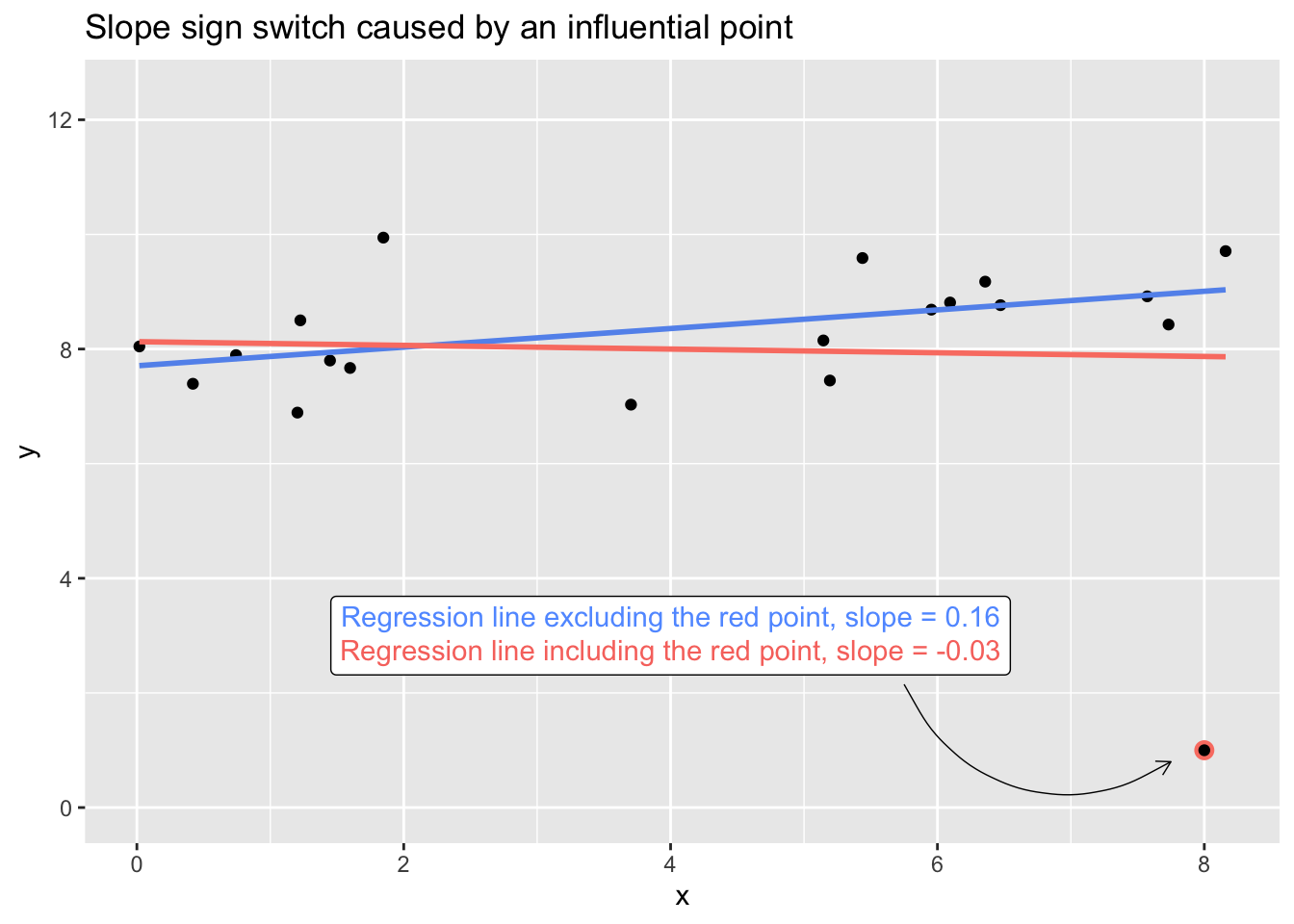
Or say that all points are in fact accurately recorded, but one of the respondents (the observation with \(y = 1\)) has a radically suppressed value of \(y\) because of a medication they’re taking at the time of measurement. The inclusion of their data during modeling would lead me to misestimate the relationship between \(x\) and \(y\).

To be clear, the goal of detecting influential points is not simply to identify data points to toss out in order to build a “clean” model or a model that accommodates the analyst’s preconceptions and expectations. Identifying influential points should motivate transparency about the fragility of a regression’s results: If a model is sufficiently fragile that the removal of an observation would meaningfully alter one’s conclusions, that should be made apparent, as should the method of addressing influential points (if action is taken), whether that be the correction of a data-entry error, the removal of an observation, or the respecification of a model. And reporting model results with and without highly influential points—so that readers can examine the fragility of a model’s results themselves—is always welcome.

One useful metric for evaluating the influence of a given observation is DFBETA. DFBETA has a delightfully simple meaning: It’s the change in a regression coefficient when the \(i^{th}\) observation is removed. For a single observation, we can calculate \(p\) DFBETA values, where \(p\) is the number of estimated parameters in the regression model (i.e., the number of predictor variables plus one, as we can also assess how the intercept estimate, \(\hat{\beta_0}\), changes upon removal of the \(i^{th}\) point).

The DFBETA for the \(j^{th}\) coefficient for the \(i^{th}\) observation is:

\[DFBETA_{ij} = \hat{\beta_j} - \hat{\beta}_{(i)j}\] Where:

• \(\hat{\beta_j}\) is the \(j^{th}\) coefficient from the regression calculated using all the data
• \(\hat{\beta}_{(i)j}\) is the \(j^{th}\) coefficient from the regression calculated without the \(i^{th}\) observation

For linear regression models, DFBETA values are usually calculated via equations that relate the least-squares fit of a model calculated with \(n\) observations to the fit with \(n-1\) observations (as opposed to recalculating the full model \(n\) times) (Belsley et al., 1980, p. 13).

It’s also reasonable to take the absolute value of each difference and not worry about the order of the subtracted elements:

\[|DFBETA_{ij}| = |\hat{\beta_j} - \hat{\beta}_{(i)j}| = |\hat{\beta}_{(i)j} - \hat{\beta_j}|\] The scale of a DFBETA value depends on the scale of the variables in the model. (The DFBETA values for a model predicting weight from height will, of course, vary depending on whether height is in feet or meters and whether weight is in pounds or kilograms.) Consequently, some analysts opt to standardize DFBETA values—in which case they’re referred to as DFBETAS—by dividing each DFBETA by the standard error estimate for \(\hat{\beta_j}\). For linear regression models, the calculation is as follows, with the error variance used in the standard error estimate replaced with the error variance from the \(i^{th}\)-deleted regression (Belsley, 1980, pp. 11–14; Li & Valliant, 2011):

\[DFBETAS_{ij} = \frac{\hat{\beta_j} - \hat{\beta}_{(i)j}}{SE(\hat{\beta}_{j})} = \frac{\hat{\beta_j} - \hat{\beta}_{(i)j}}{\sqrt{MSE_{(i)} \times C_{jj}}}\]

Where:

• \(MSE_{(i)}\) is the mean squared error of the regression calculated without the \(i^{th}\) observation
• \(C_{jj}\) is the \(j^{th}\) diagonal element of \((X'X)^{-1}\) matrix of the regression calculated with all observations

DFBETA and DFBETAS values can be calculated for many models in R with the dfbeta() and dfbetas() functions, respectively. (DFBETAS values are also calculated by the general influence.measures() function, which returns them alongside a number of other diagnostics.) Once DFBETA or DFBETAS values have been calculated, the challenge of determining which points are influential enough to warrant follow-up is in the hands of the analyst. No perfect cutoff exists, but a common threshold against which to compare |DFBETAS| values is \(\frac{2}{\sqrt{n}}\) (Belsley et al., 1980, p. 28). This is a size-adjusted threshold, as in a sample of 1000, a given point will have less influence than in a sample of 100, all else equal. In the former case, the impact of even a high-leverage, high-outlyingness point is “drowned out” by the other points. But it’s helpful to still be able to identify points that are relatively influential; the \(\frac{2}{\sqrt{n}}\) formula calibrates the threshold to the sample size used to construct the model. With \(n = 100\), the loose |DFBETAS| threshold for an influential point would be \(\frac{2}{\sqrt{100}} = 0.20\), or one-fifth of the standard error estimate for the corresponding coefficient, whereas with \(n = 1000\), the threshold drops to \(\frac{2}{\sqrt{1000}} = 0.063\), or approximately one-sixteenth of the standard error estimate for the corresponding coefficient. Belsley et al. describe the size-adjusted criterion as one that “expose[s] approximately the same proportion of potentially influential observations, regardless of sample size” (1980, p. 28).

With anything but a small \(n\), inspecting DFBETA or DFBETAS values individually becomes an arduous task. Instead, one can generate a plot with observation indexes on the x-axis and DFBETA(S) values on the y-axis. If the analyst has a threshold in mind, they can overlay that on the plot and identify influential points to examine based on which approach or exceed the line. For example, below I simulate \(x\) and \(y\) values for 100 observations, where \(x\) is randomly drawn from a uniform distribution, \(U(10, 100)\), and \(y\) is given by the data-generating process \(y = 2 + 1.25x + e,~e \sim N(0, 100)\). I then inflate the \(y\)-value of 10 randomly selected observations by further multiplying each one by 2. I then model \(y\) as a linear function of \(x\) and manually generate a plot of the DFBETAS values for \(x\) for each observation. The plot includes thresholds at \(\pm\frac{2}{\sqrt{n}}\).

# Simulate data
set.seed(2022^2)
x <- runif(100, min = 10, max = 100)
y <- 2 + 1.25*x + rnorm(100, mean = 0, sd = 10)
# Randomly pick 10 observations for which to inflate y
to_inflate <- sample(length(y), 10, replace = F)
# Inflate
y[to_inflate] <- y[to_inflate] * 2

# Model
mod <- lm(y ~ x)

# DFBETAS values (placing them in a data frame ensures easy compatibility with ggplot2)
dfbetas_vals <- data.frame(dfbetas(mod))

# Plot
library(ggplot2)
ggplot(dfbetas_vals) +
  geom_point(aes(x = 1:nrow(dfbetas_vals), y = x)) +
  geom_segment(aes(x = 1:nrow(dfbetas_vals), xend = 1:nrow(dfbetas_vals), y = 0, yend = x),
               color = 'cornflowerblue') +
  geom_hline(yintercept = c(2, -2) / sqrt(nrow(dfbetas_vals)), color = 'salmon') +
  labs(x = 'Observation index', y = 'DFBETAS',
       title = paste0('DFBETAS values for coefficient of ', colnames(dfbetas_vals)[2]),
       subtitle = 'Thresholds are at \u00B1(2\u00F7\u221An)') +
  geom_text(aes(x = 1:nrow(dfbetas_vals), y = ifelse(x > 0, x + .05, x - .05),
                label = ifelse(abs(x) > (2/sqrt(nrow(dfbetas_vals))),
                               paste0(round(x, digits = 2), ' (', 1:nrow(dfbetas_vals), ')'), '')))

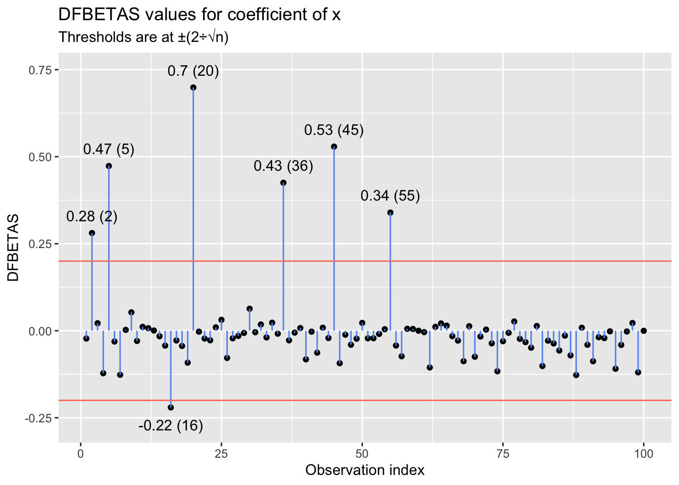
The plot suggests that several points have a sizable influence on the slope estimate for \(x\). In this case, visual inspection of the linear relationship between \(x\) and \(y\) is possible, and inspection reinforces what was suggested by the DFBETAS values: It appears that a subset of the points—the ones peeling up and away from the primary linear trend—follow a different data-generating process than the rest. And, of course, we know that they do: \(y = 2(2 + 1.25x + e),~e \sim N(0, 100)\). Those points drag the slope for \(x\) upward (they affect the intercept as well, although I focus here on impacts on the slope).

plot(x, y)
abline(mod)
abline(lm(y[-to_inflate] ~ x[-to_inflate]), col = 'salmon')
text(x = 45, y = 250, labels = 'Salmon line is regression line omitting inflated points')

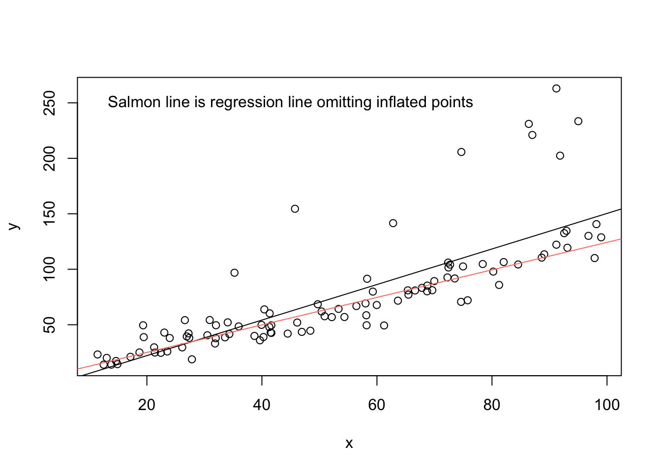
Direct visual inspection as above often isn’t possible in analyses with multiple predictors (e.g., \(\hat{y} = \hat{\beta}_0 + \hat{\beta}_1x_1 + \hat{\beta}_2x_2 + ... + \hat{\beta}_jx_j\)). In those cases, we rely on metrics like DFBETA(S) to help identify influential points that warrant follow-up.

In the example above, I created a plot of the DFBETAS values manually with ggplot2 in order to apply some custom controls. There are, though, several functions on offer in various packages that generate similar plots automatically; those include:

# Plots DFBETAS values for all model terms (intercept and predictors), as well as +/- 2/sqrt(n) cut-offs
olsrr::ols_plot_dfbetas(mod)
# Plots DFBETAS values for all model terms except for the intercept
car::dfbetasPlots(mod)
# Plots DFBETA values for all model terms except for the intercept
car::dfbetaPlots(mod)

I mentioned before that the common \(\frac{2}{\sqrt{n}}\) threshold for |DFBETAS| values is intended to identify a similar proportion of influential points across different sample sizes for a given model. We can demonstrate this via simulation to spark the intuition. Below, I simulate 1000 data sets with sample sizes \(n = 10, 20, 30,..., 10000\). In each, I simulate a vector of \(x\) values by drawing randomly from a uniform distribution, \(U(10, 100)\), and I simulate a vector of \(y\) values given by the data-generating process \(y = 2 + 1.25x + e, e \sim N(0, 100)\). I fit a linear model, \(\hat{y} = \hat{\beta}_0 + \hat{\beta}_1x\), and then calculate the DFBETAS value for each parameter estimate for each observation. Finally, in each data set, I calculate the proportion of |DFBETAS| values for each parameter estimate (\(\hat{\beta}_0\) and \(\hat{\beta}_1\)) that exceed a size-adjusted threshold, \(\frac{2}{\sqrt{n}}\), and that exceed a fixed threshold, 0.05 (1/20th of a standard error estimate of \(\hat{\beta}_j\).) The proportions of |DFBETAS| values that exceed each threshold for each coefficient across varying sample sizes are shown in the plots.

ns <- seq(from = 10, to = 10000, by = 10)
proportion_exceeding <- data.frame(x_flexthresh = vector(length = length(ns)),
                                   Intercept_flexthresh = vector(length = length(ns)),
                                   x_fixthresh = vector(length = length(ns)),
                                   Intercept_fixthresh = vector(length = length(ns)))

for (i in 1:length(ns)) {
  x <- runif(ns[i], min = 10, max = 100)
  y <- 2 + 1.25*x + rnorm(ns[i], 0, 10)
  mod <- lm(y ~ x)
  proportion_exceeding$x_flexthresh[i] <- sum(abs(dfbetas(mod)[, 2]) > (2 / sqrt(ns[i]))) / ns[i]
  proportion_exceeding$Intercept_flexthresh[i] <- sum(abs(dfbetas(mod)[, 1]) > (2 / sqrt(ns[i]))) / ns[i]
  proportion_exceeding$x_fixthresh[i] <- sum(abs(dfbetas(mod)[, 2]) > .05) / ns[i]
  proportion_exceeding$Intercept_fixthresh[i] <- sum(abs(dfbetas(mod)[, 1]) > .05) / ns[i]
}

proportion_exceeding_long <- tidyr::pivot_longer(proportion_exceeding,
                                                 cols = everything(),
                                                 values_to = 'proportion',
                                                 names_to = c('coefficient', 'threshold_type'),
                                                 names_pattern = '(.+)_(.+)')

ggplot(proportion_exceeding_long) +
  geom_point(aes(x = 1:nrow(proportion_exceeding_long)/4, y = proportion, color = threshold_type),
             size = .5) +
  geom_line(aes(x = 1:nrow(proportion_exceeding_long)/4, y = proportion, color = threshold_type),
            alpha = .5, lwd = .25) +
  scale_x_continuous(breaks = seq(1, length(ns), by = 200), labels = ns[seq(1, length(ns), by = 200)]) +
  scale_color_manual('Threshold', labels = c('Fixed: 0.05', 'Dynamic: \u00B1(2\u00F7\u221An)'),
                     values = c('salmon', 'cornflowerblue')) +
  facet_wrap(~coefficient) +
  labs(x = 'n', y = 'Proportion',
       title = paste0('Proportion of |DFBETAS| values for each coefficient that exceed',
                      '\nthreshold across varying sample sizes and threshold types'),
       subtitle = paste0('True data-generating process: y = 2 + 1.25x + e, ',
                         'e ~ N(0, 100), x ~ U(10, 100)',
                         '<br>Model fit: y = \u03B2<sub>0</sub> + \u03B2<sub>1</sub>x')) +
    theme(plot.subtitle = ggtext::element_markdown())

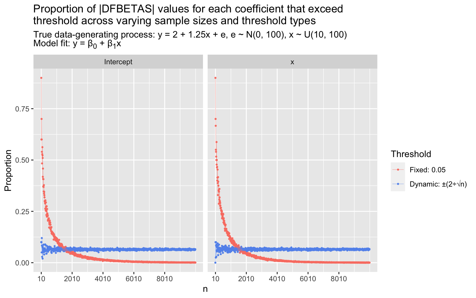
As \(n\) increases, the proportion of points with |DFBETAS| values that exceed the fixed threshold (0.05) collapses toward zero. The proportion is largely determined by \(n\). Conversely, the proportion of points with |DFBETAS| values that exceed the size-adjusted threshold, \(\frac{2}{\sqrt{n}}\), stabilizes around ~0.065 (the exact proportion will vary model to model). The proportion flagged by the size-adjusted threshold actually gets more stable as \(n\) increases (as described in Li & Valliant, 2011): Fanning that’s apparent in the \(n < 1000\) range is compressed toward a stable line at higher \(n\)s. The absolute effects of any given point on the intercept and slope estimates get smaller as \(n\) increases, so if identifying absolutely influential points is the goal, the fixed threshold is preferable; but if the aim is to identify relatively influential points, the size-adjusted threshold does a superior job.

I’ve so far discussed DFBETA(S) values in the context of linear regression models. These influence measures can also be used when working with generalized linear models, like logistic regressions. For example, say I fit a logistic regression using R’s built-in mtcars data set predicting whether vehicles have automatic (am == 0) or manual (am == 1) transmissions from their gas mileage (mpg).

mod <- glm(am ~ mpg, data = mtcars, family = 'binomial')
coef(mod)

(Intercept)         mpg 
 -6.6035267   0.3070282 

DFBETA and DFBETAS values, then, are on the log odds and standardized log odds scales, respectively.

head(dfbeta(mod), n = 3)

              (Intercept)         mpg
Mazda RX4     -0.02280558 0.007871482
Mazda RX4 Wag -0.02280558 0.007871482
Datsun 710    -0.27448276 0.019173841

head(dfbetas(mod), n = 3)

               (Intercept)        mpg
Mazda RX4     -0.009863448 0.06970744
Mazda RX4 Wag -0.009863448 0.06970744
Datsun 710    -0.117613781 0.16822375

Note, though, that DFBETA(S) values for generalized linear models are approximations. As mentioned above, DFBETA(S) calculations for linear regressions rely on equations that relate the least-squares fit of a model with \(n\) observations to the least-squares fit with \(n-1\) observations. These methods don’t apply in the case of generalized linear models: As Williams (1987) describes, “The maximum likelihood (ML) estimation of most generalized linear models (GLMs) requires iterative methods. The ML estimates from \(n-1\) cases cannot then be obtained as explicit functions of the results of the fit to all \(n\) cases.” The documentation for dfbeta() and dfbetas() indicates that the values those functions calculate for models fit with glm() are based on methods described in Williams (1987). Similar complications apply in the case of multilevel/mixed-effects linear and generalized linear models (like those fit with the lme4 package), as those models are also estimated with iterative techniques (ML/REML). lme4 provides methods for calculating DFBETA(S) values for mixed-effects linear and generalized linear models: A user can pass an lme4 model to influence() and then pass the resulting object to dfbeta() or dfbetas().

DFBETA(S) values can also be used to understand influence in non-linear models, such as the polynomial regression \(\hat{y} = \hat{\beta}_0 + \hat{\beta}_1x + \hat{\beta}_2x^2\). Say that I draw 1000 \(x\) values from a uniform distribution, \(U(1, 10)\), and I generate 1000 \(y\) values via the data-generating process \(y = 2 + 0.5x + 1.25x^2 + e,~e \sim N(0, 1)\). I then estimate the following model: \(\hat{y} = \hat{\beta}_0 + \hat{\beta}_1x + \hat{\beta}_2x^2\).

x <- runif(1000, 1, 10)
x2 <- x^2
y <- 2 + 0.5*x + 1.25*x2 + rnorm(1000, mean = 0, sd = 1)

mod <- lm(y ~ x + x2)
coef(mod)

(Intercept)           x          x2 
  1.9658258   0.5113185   1.2496943 

The \(\hat{\beta}_2\) coefficient on \(x^2\) characterizes the acceleration of the slope of the modeled curve relating \(x\) to \(y\), as the second derivative of the model gives the change in the curve’s slope given a unit increase in \(x\):

\[\hat{y} = 1.97 + 0.51x + 1.25x^2\]

\[\hat{y}' = 0.51 + (2)1.25x\]

\[\hat{y}'' = 2.50\]

The acceleration of the slope across values of \(x\) is visible in a plot of the points:

x3slope <- .51 + 2*1.25*3
y_at_x3 <- 1.97 + .51*3 + 1.25*3^2
x3intercept <- y_at_x3 - x3slope*3
x8slope <- .51 + 2*1.25*8
y_at_x8 <- 1.97 + .51*8 + 1.25*8^2
x8intercept <- y_at_x8 - x8slope*8

ggplot() +
  geom_point(aes(x = x, y = y), color = '#3D405B', size = .25) +
  geom_abline(aes(intercept = x3intercept, slope = x3slope), color = '#81B29A') +
  geom_abline(aes(intercept = x8intercept, slope = x8slope), color = '#E07A5F') +
  annotate('text', x = 4, y = 100,
           label = paste0('Green and red tangent lines have slopes equal to the',
                          '\nslope of the modeled curve at x = 3 (slope = ', x3slope, ')',
                          '\nand x = 8 (slope = ', x8slope, '), respectively'))

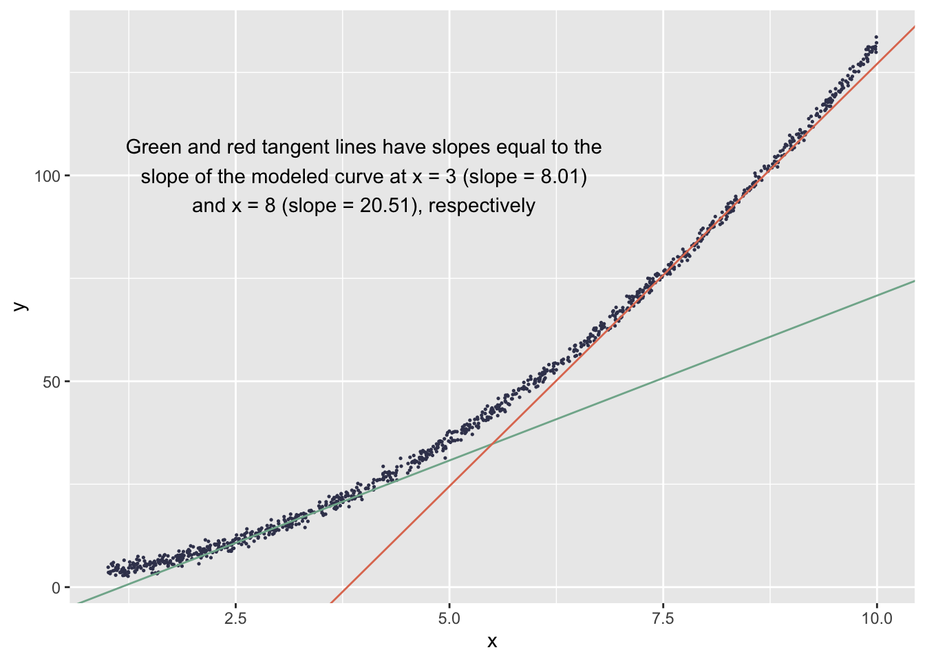
The DFBETA values for the coefficient of \(x^2\) help us understand how the slope acceleration is affected by each observation.

head(dfbeta(mod), n = 3)

    (Intercept)             x            x2
1 -3.032678e-03  2.138491e-03 -2.039613e-04
2 -1.273164e-05  1.028829e-05 -1.582270e-06
3  7.525833e-04 -2.128544e-04  1.428457e-05

range(dfbeta(mod)[, 3])

[1] -0.0006830925  0.0006840470

Given the tight range of the DFBETA values for \(\hat{\beta}_2\), it’s clear that the influence of any given point on the acceleration of the slope is minute. The second derivatives of the models fit with \(n-1\) observations would all be nearly identical to that of the model fit with \(n\) observations.

DFBETA(S) values are particularly useful if the analyst or researcher’s priority is estimating the coefficients of predictors in a regression and understanding how fragile those slopes are. There are several other influence measures that are also based on single-case deletion—most notably, DFFIT(S) and Cook’s D; those measures express how deletion of the \(i^{th}\) case affects model predictions. Those predictions are, of course, functions of coefficients, so these measures all ultimately address the same overarching question—how sensitive is the model to the removal of a given observation?—but DFFIT(S) and Cook’s D values aim the evaluative microscope at a different aspect of the model than do DFBETA(S). Influence diagnostics help researchers and analysts understand their model results holistically: A model’s parameter estimates are just that—estimates, limited by sampling error and sometimes rendered fragile by idiosyncrasies of the underlying data. They’re not etched into the Kish tablet for perpetuity, and understanding their fragility is important for fully understanding a model.

References

• Belsley, D. A., Kuh, E., & Welsch, R. E. (1980). Regression diagnostics: Identifying influential data and sources of collinearity. John Wiley & Sons.
• Li, J., & Valliant, R. (2011). Linear regression influence diagnostics for unclustered survey data. Journal of Official Statistics, 27(1), 99–119.
• Williams, D. (1987). Generalized linear model diagnostics using the deviance and single case deletions. Journal of the Royal Statistical Society: Series C (Applied Statistics), 36(2), 181–191.

Jacob Goldstein-Greenwood
Research Data Scientist
University of Virginia Library
July 29, 2022