
R users who have run base R’s prop.test() function to perform a null hypothesis test of a proportion—as when assessing whether a coin is weighted toward heads or whether more than half of the wines a vineyard sold in a given month were reds—may have noticed curious language in the output: The default test is reported as having been performed with a “continuity correction.”
# One-sided one-sample proportion test
set.seed(999)
dat <- rbinom(1, 50, .6)
prop.test(dat, n = 50, p = .5, alternative = 'greater')
    1-sample proportions test with continuity correction
data:  dat out of 50, null probability 0.5
X-squared = 2.42, df = 1, p-value = 0.0599
alternative hypothesis: true p is greater than 0.5
95 percent confidence interval:
 0.4937005 1.0000000
sample estimates:
   p
0.62
From the output alone, it’s not immediately clear what is purportedly being corrected, what the precise method of correction is, or if a correction is even warranted.
Continuity corrections are adjustments that can be made to statistical tests when discontinuous distributions (like binomial distributions) are approximated by continuous ones (like normal distributions). These approximations can be fairly accurate, and historically—before computing power was widespread—they were time-savers. “Fairly accurate,” however, is not “perfectly accurate”; approximations involve error, and the development of continuity corrections was an effort to account for that fact.
Say, for example, that I perform a one-sample proportion test to assess whether a coin is biased in favor of heads. In reality (although unbeknownst to me), the coin is indeed unfair—there’s a 60% chance that it lands obverse-up. I flip the coin 50 times and observe 29 heads:
# Flip a biased coin 50 times (true probability of heads = .60)
heads <- rbinom(n = 1, size = 50, prob = .60)
heads
[1] 29
The aim of the test is to figure out how surprising the 29 observed heads would be if the coin was fair. The probability distribution of heads for a fair coin that’s flipped 50 times is a binomial distribution defined by parameters n (50) and p (0.5). Binomial distributions are decently approximated by normal distributions at more-than-minute sample sizes.1 The approximate normal distribution’s mean is \(np\), and its standard deviation is \(\sqrt{np(1 - p)}\). (And since the counts are approximately normally distributed, so are the corresponding proportions—the counts divided by the sample size: The mean of the distribution of proportions is p, and the standard deviation is \(\sqrt{\frac{p(1-p)}{n}}\).)
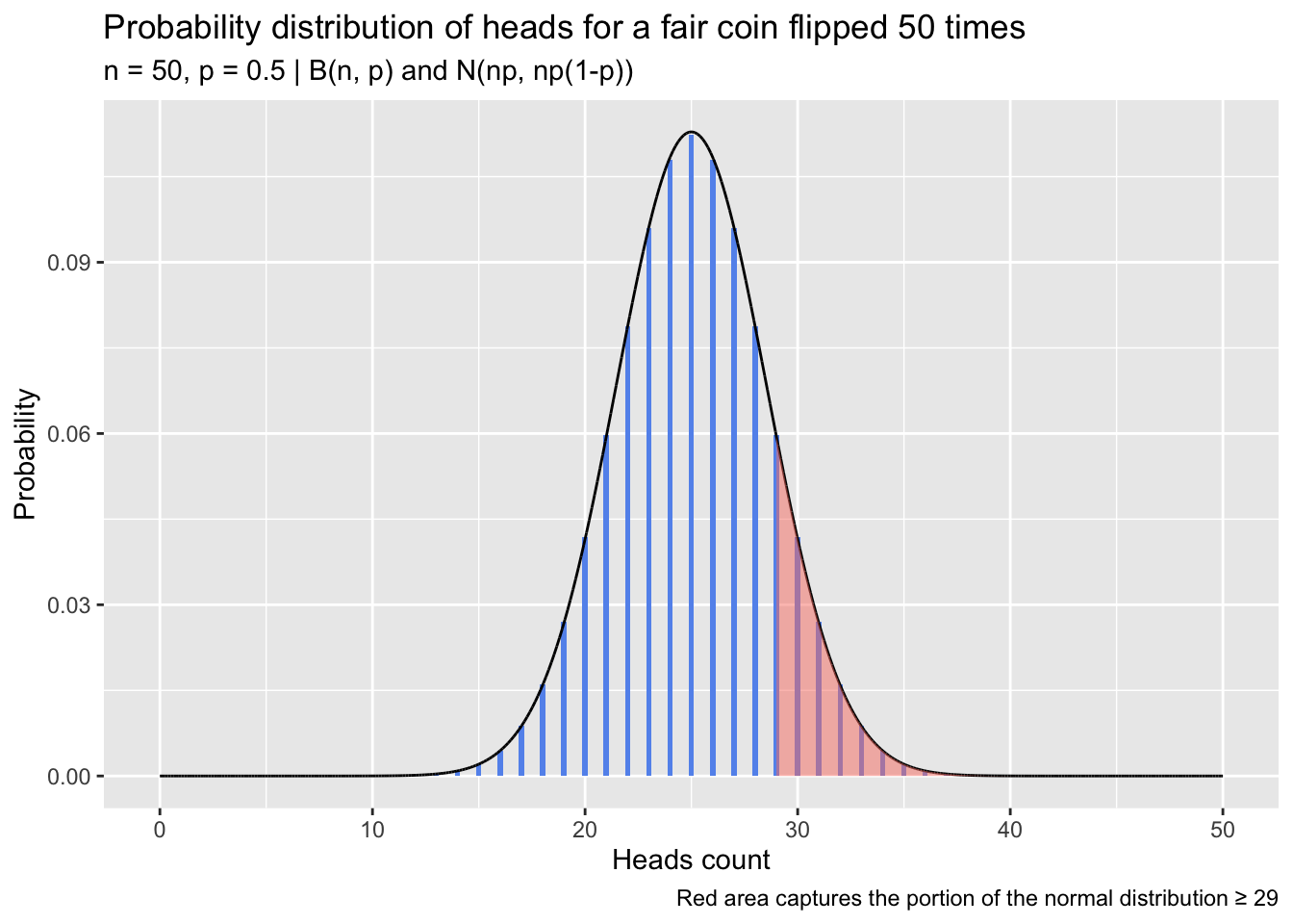
One calculates the probability of observing at least 29 heads in 50 flips if handling a fair coin. This can be achieved by identifying where the observed count (or proportion) of heads falls in the approximate normal distribution itself, or by calculating a z statistic from the observed count (or proportion) and referencing a standard normal distribution. The binomial distribution of heads for a fair coin (p = 0.5) is shown in the following plot with the corresponding approximate normal distribution overlaid. The portion of the normal distribution greater than or equal to 29 is shaded red. Probability calculations follow the plot.
library(ggplot2)
n = 50; p = 0.5
binom <- data.frame(count = 0:n, y = dbinom(x = 0:n, size = n, prob = p))
norm_dat <- data.frame(x = seq(0, n, by = .001), y = dnorm(seq(0, n, by = .001), n*p, sqrt(n*p*(1-p))))
ggplot(binom, aes(count, y)) +
  geom_col(fill = 'cornflowerblue', width = .25) +
  geom_line(data = norm_dat, aes(x = x, y = y)) +
  labs(title = 'Probability distribution of heads for a fair coin flipped 50 times',
       subtitle = 'n = 50, p = 0.5 | B(n, p) and N(np, np(1-p))',
       x = 'Heads count', y = 'Probability',
       caption = 'Red area captures the portion of the normal distribution \u2265 29') +
  geom_area(data = norm_dat[norm_dat$x >= heads, ], aes(x = x, y = y),
            fill = 'salmon', alpha = .5)
# Calculate the probability based on the approximate normal null distribution of heads counts
flips <- 50
proportion_heads <- heads / flips
null_proportion <- .5
pnorm(q = heads, mean = flips*null_proportion, sd = sqrt(flips*null_proportion*(1-null_proportion)),
      lower.tail = F)
[1] 0.1289495
# Alternatively and equivalently:
# Calculate the probability by calculating a z-value and comparing it to a standard normal distribution
se <- sqrt((null_proportion * (1 - null_proportion)) / flips)
z <- (proportion_heads - null_proportion) / se
pnorm(z, lower.tail = F)
# Or via prop.test()
prop.test(x = heads, n = flips, p = null_proportion, alternative = 'greater', correct = F)$p.value
Using the normal approximation isn’t obligatory: The probability can, alternatively, be exactly calculated for this test from the binomial distribution—the true null sampling distribution. To do so, one sums the probabilities in the relevant binomial distribution from 29 up to the number of flips (50). This is an “exact” null hypothesis test:
sum(dbinom(x = heads:flips, size = flips, prob = null_proportion))
[1] 0.1611182
# Alternatively and equivalently:
pbinom(q = 28, size = flips, p = null_proportion, lower.tail = F) # Use q = 28 to get probability >= 29
# Or via binom.test()
binom.test(heads, n = flips, p = null_proportion, alternative = 'greater')$p.value
Here, the probability estimated using the normal approximation and the exact probability calculated from the binomial distribution are reasonably close: 0.129 and 0.161. In the grand scheme of p-values (which should be regarded as rough estimates subject to sizable variation, not as diamonds), these aren’t worlds apart. Before the advent of widespread computing power, using normal approximations for tests like this was a welcome convenience, as calculating exact probabilities from binomial distributions was comparatively laborious: One would have to calculate and then sum the probabilities in a null binomial distribution for each of the values equal to or more extreme than one’s sample value.
But approximations come with error, and the error can be sizable, especially when working with small sample sizes. Below, I simulate flipping a fair coin at a range of “flip counts,” performing 2500 trials at each one. On each trial, I perform a pair of one-sample proportion tests comparing the observed proportion against a null of 0.5; the first test uses the normal approximation, and the second uses the binomial distribution directly. The tests give the probability of observing at least the number of heads in that trial if the coin was indeed fair. I compute the ratio of those probabilities—normal-approximation p-value divided by exact binomial p-value—on each trial. A plot showing how the distribution of ratios changes depending on the number of flips performed in each trial is below.
set.seed(2023)
flips <- seq(10, 250, by = 10)
times <- 2500
p_dat <- data.frame(matrix(NA, nrow = times, ncol = length(flips)))
colnames(p_dat) <- flips
calculate_ratio <- function(flips, true_heads_prob = .50, null_prob = 0.5,
                            alt = 'greater', correct = FALSE) {
  heads <- rbinom(n = 1, size = flips, prob = true_heads_prob)
  normal_approx <- prop.test(heads, n = flips, p = null_prob, alternative = alt, correct = correct)
  binom <- binom.test(heads, n = flips, p = null_prob, alternative = alt)
  normal_approx$p.value / binom$p.value
}
for (i in 1:length(flips)) { p_dat[, i] <- replicate(times, calculate_ratio(flips[i])) }
p_dat <- tidyr::pivot_longer(p_dat, cols = dplyr::everything(),
                             names_to = 'flips', values_to = 'p_ratio',
                             names_transform = as.integer)
medians <- aggregate(p_dat$p_ratio, by = list(p_dat$flips), median)
colnames(medians) <- c('flips', 'median_val')
ggplot(p_dat, aes(flips, p_ratio, group = flips)) +
  geom_line(data = medians, aes(flips, median_val, group = 1), col = 'cornflowerblue') +
  geom_violin(fill = 'salmon', alpha = .5) +
  labs(title = expression(paste('Ratios of normal-approximation test ', italic(p),
                                '-values to exact binomial test ', italic(p),
                                '-values across flip counts')),
       subtitle = paste0('One-sided one-sample proportion test performed 2500 times at each flip count',
                         '\nBlue line tracks median ratio at each flip count'),
       x = 'Flip count', y = expression(italic(p)~'ratio'),
       caption = paste0("No continuity correction used in normal-approximation tests",
                        "\nNull heads probability and coin's true heads probability ",
                        "are both 0.5 in all trials")) +
  ylim(0.5, 1.50)
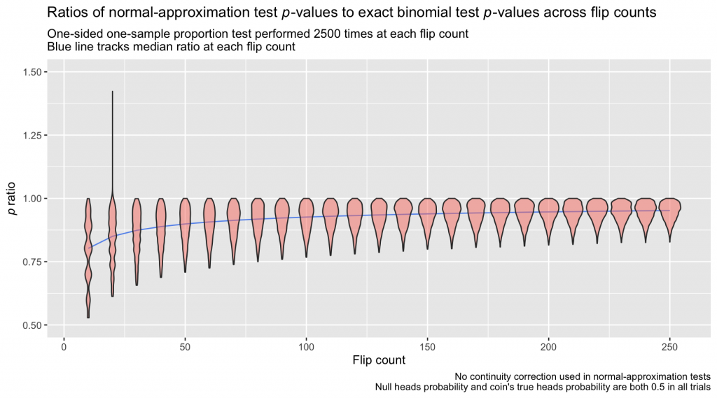
The bulk of normal-approximation test p-values in this example are low compared to the p-values from the exact binomial tests, and the underestimation is severe at low sample sizes, with ratios dipping down almost to 0.5. A continuity correction aims to bring these values more in line and reduce the error introduced by the normal approximation. The adjustment itself is simple; instead of calculating \(P(X \ge x)\) or \(P(X \le x)\) in the normal distribution, one subtracts or adds 0.5 from x depending on the direction of the test:
- For a one-sided “greater than” test, one calculates \(P(X \ge x - 0.5)\) instead of \(P(X \ge x)\)
- For a one-sided “less than” test, one calculates \(P(X \le x + 0.5)\) instead of \(P(X \le x)\)
- For a two-sided test, one calculates two times the 0.5-adjusted one-sided probability
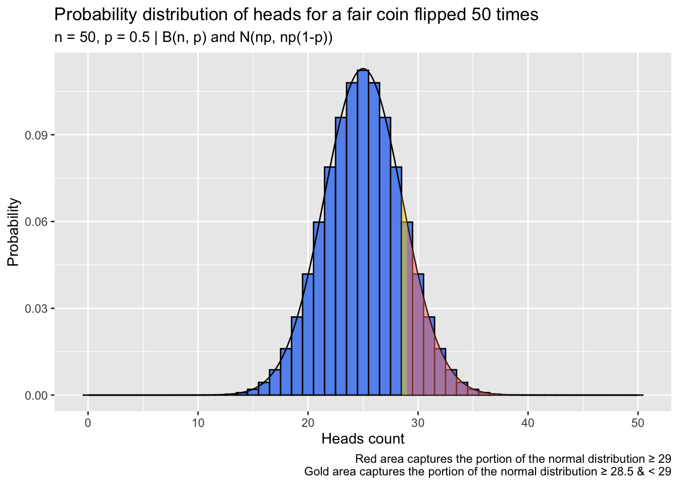
This inflates the probability calculated via normal approximation somewhat, with the aim of bringing it closer to the exact probability calculated from the binomial distribution. The selection of 0.5 as the adjustment value isn’t arbitrary: Probabilities in the binomial distribution lie only at integer values—counts—whereas a normal distribution expresses probabilities for the continuous span of values between each pair of integers. If we imagine taking the null binomial distribution from the first example, \(B(50,0.5)\), and spreading its probability out to cover the same continuous span of values as its approximate normal cousin, we’d obtain a distribution with “bins” as below. The bin for x = 29 (the observed heads count in that example) begins at 28.5. We can think of half of the interval between 28 and 29 as “belonging” to 29, and the continuity correction captures that half-interval:
ggplot(binom, aes(count, y)) +
  geom_col(fill = 'cornflowerblue', color = 'black', width = 1) +
  geom_line(data = norm_dat, aes(x = x, y = y)) +
  labs(title = 'Probability distribution of heads for a fair coin flipped 50 times',
       subtitle = 'n = 50, p = 0.5 | B(n, p) and N(np, np(1-p))',
       x = 'Heads count', y = 'Probability',
       caption = paste0('Red area captures the portion of the normal distribution \u2265 29\n',
                        'Gold area captures the portion of the normal distribution ',
                        '\u2265 28.5 & \u003C 29')) +
  geom_area(data = norm_dat[norm_dat$x >= heads, ], aes(x = x, y = y),
            fill = 'salmon', alpha = .5) +
  geom_area(data = norm_dat[norm_dat$x >= 28.5 & norm_dat$x < heads, ], aes(x = x, y = y),
            fill = 'gold', alpha = .5)
How much does this adjustment affect estimates? Below, I repeat the coin-flipping simulation from before, this time applying the continuity correction to the normal-approximation test before calculating the p ratio on each trial:
p_dat <- data.frame(matrix(NA, nrow = times, ncol = length(flips)))
colnames(p_dat) <- flips
for (i in 1:length(flips)) { p_dat[, i] <- replicate(times, calculate_ratio(flips[i], correct = TRUE)) }
p_dat <- tidyr::pivot_longer(p_dat, cols = dplyr::everything(),
                             names_to = 'flips', values_to = 'p_ratio',
                             names_transform = as.integer)
medians <- aggregate(p_dat$p_ratio, by = list(p_dat$flips), median)
colnames(medians) <- c('flips', 'median_val')
ggplot(p_dat, aes(flips, p_ratio, group = flips)) +
  geom_line(data = medians, aes(flips,median_val, group = 1), col = 'cornflowerblue') +
  geom_violin(fill = 'salmon', alpha = .5) +
  labs(title = expression(paste('Ratios of normal-approximation test ', italic(p),
                                '-values to exact binomial test ', italic(p),
                                '-values across flip counts')),
       subtitle = paste0('One-sided one-sample proportion test performed 2500 times at each flip count',
                         '\nBlue line tracks median ratio at each flip count'),
       x = 'Flip count', y = expression(italic(p)~'ratio'),
       caption = paste0("Continuity correction used in normal-approximation tests",
                        "\nNull heads probability and coin's true heads probability ",
                        "are both 0.5 in all trials",
                        "\nSix ratios extending beyond the y-axis of the plot ",
                        "(all \u2265 1.5 and at flip counts \u2264 30) are not shown")) +
    ylim(0.5, 1.50)
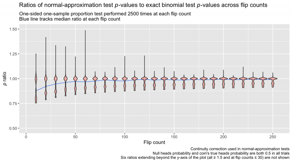
The continuity-corrected normal-approximation p-values are again imperfect, but the bulk of the ratios lie closer to 1.0 than in the first simulation, which omitted the continuity correction. At relatively large sample sizes, the differences between the continuity-corrected normal-approximation probabilities and the probabilities calculated directly from the binomial distribution are practically negligible.
There are still, however, troubling deviations from a ratio of 1.0 at small sample sizes, and that residual risk of error motivates me to use an exact binomial test when performing a one-sample proportion test, especially with a small N. Further, the continuity correction does not have the unilateral effect of compressing underestimated normal-approximation p-values toward their exact binomial test counterparts: When the sample proportion being tested is far into the tail of the null distribution, the correction can lead to overestimation of the p-value (relative to the p-value from the corresponding exact binomial test; Richardson, 1994). This phenomenon is apparent in the plot above where the violin bodies exceed 1.0 (some trials, as a consequence of random sampling, have heads proportions that far exceed or undershoot 0.5 and thus land deep in one of the null distribution’s tails). Note too that the accuracy of a normal approximation of a binomial distribution decays as the probability of the event reflected in the distribution deviates from 0.5, and the improving effect of the continuity correction is worse in those cases; inaccuracies introduced by normal approximation are often left unresolved. In the occasional circumstance where I look to test a sample proportion against a null proportion of 0.1, 0.9, or some similar far-from-0.5 value, I again prefer an exact binomial test: Why attempt to correct a sizable estimation error when the error can be avoided in the first place?
Historically, some analysts have also used a continuity correction when comparing a pair of sample proportions with a \(\chi^2\) test of association for a 2x2 contingency table. A \(\chi^2\) distribution is continuous, but the values filling a contingency table are discrete counts, rendering the distribution of the test statistic not truly continuous. This can result in a slight overestimation of the \(\chi^2\) test statistic (and thus a slight underestimation of the p-value of the test). Some analysts apply “Yates’s continuity correction” (Yates, 1934) in response by modifying the calculation of the Pearson’s \(\chi^2\) test statistic from \(\chi^2 = \sum_{i=1}^r\sum_{j=1}^c\frac{(O_{ij} - E_{ij})^2}{E_{ij}}\) to \(\chi^2 = \sum_{i=1}^r\sum_{j=1}^c\frac{(|O_{ij} - E_{ij}| - 0.5)^2}{E_{ij}}\). This modification, though, has been justifiably criticized: Monte Carlo simulations suggest that the continuity correction is extremely conservative when working with 2x2 tables (e.g., Camilli & Hopkins, 1978; Grizzle, 1967; Richardson, 1990), and the modification has the effect of making the p-value from a \(\chi^2\) test of association more-closely approximate the p-value from a Fisher’s exact test, even though the underlying premise of a Fisher’s exact test—that the row and column totals of a contingency table are fixed, not subject to sampling—is rarely satisfied in the wild (Haviland, 1990; Stefanescu et al., 2014). For analyses of 2x2 contingency tables in which expected cell values (\(E_{ij}\)) are at least approximately 1.0, Pearson’s \(\chi^2\) test without a continuity correction maintains close to the nominal Type I error rate, even with fairly small total sample sizes (Camilli & Hopkins, 1978; see also a discussion and references from biostatistician Frank Harrell here).
This all can leave the analyst in a curious, unsure position. A “correction” seems reflexively desirable, and continuity corrections are applied by default by base R functions like prop.test() and chisq.test(). But nowadays, continuity corrections are arguably of limited use. In the case of a one-sample proportion test, the aim of the correction is to make normal-approximation p-values better approximate those from exact binomial tests, and in the days when exact binomial tests were difficult to perform given their sheer computational toll, this was a helpful adjustment. But exact binomial tests take mere moments with contemporary computing power,2 and given that the continuity correction still risks sizable error—especially when working with small sample sizes, sample proportions near 0 or 1.0, and/or null proportions far from 0.5—I generally prefer exact binomial tests. In the case of a two-sample proportion test in which, as is common, the row and column totals aren’t fixed (i.e., a Pearson’s \(\chi^2\) test of a 2x2 contingency table), Yates’s continuity correction is so conservative as to be effectively impossible to recommend (Lydersen et al., 2009)—it bludgeons the Type I error rate of the test down well below the nominal level. That conservatism doesn’t serve the admirable aim of scientific caution: Far better for nominal Type I error rates to mean what they advertise. If an analyst wishes to restrict her Type I error rate in a frequentist testing framework, she can lower her “significance” threshold (\(\alpha\)); the test need not dip away from the stated rate without warning.
The subtle problem that continuity corrections were developed to address—error introduced by approximating discontinuous distributions with continuous ones—is not imaginary, but their utility is depressed by access to modern computing power (which makes exact binomial tests easy to perform when assessing one proportion against a null) and by their conservatism (when comparing a pair of sample proportions). Seeing as common R functions like prop.test() and chisq.test() apply continuity corrections by default, it’s worth understanding what they are—but understanding entails no obligation.
R session details
The analysis was verified using the R Statistical language (v4.5.2; R Core Team, 2025) on Windows 11 x64, using the packages ggplot2 (v4.0.1).
References
- Camilli, G., & Hopkins, K. D. (1978). Applicability of chi-square to 2×2 contingency tables with small expected cell frequencies. Psychological Bulletin, 85(1), 163–167. https://doi.org/10.1037/0033-2909.85.1.163
- Grizzle, J. E. (1967). Continuity correction in the \(\chi^2\)-test for 2x2 tables. The American Statistician, 21(4), 28–32. https://doi.org/10.2307/2682103
- Haviland, M. G. (1990). Yates’s correction for continuity and the analysis of 2×2 contingency tables. Statistics in Medicine, 9(4), 363–367. https://doi.org/10.1002/sim.4780090403
- Lydersen, S., Fagerland, M. W., & Laake, P. (2009). Recommended tests for association in 2×2 tables. Statistics in Medicine, 28(7), 1159–1175. https://doi.org/10.1002/sim.3531
- Richardson, J. T. (1990). Variants of chi‐square for 2×2 contingency tables. British Journal of Mathematical and Statistical Psychology, 43(2), 309–326. https://doi.org/10.1111/j.2044-8317.1990.tb00943.x
- Richardson, J. T. (1994). The analysis of 2x1 and 2x2 contingency tables: An historical review. Statistical Methods in Medical Research, 3(2), 107–133. https://doi.org/10.1177/096228029400300202
- Stefanescu, C., Berger, V. W., & Hershberger, S. L. (2014). Yates’ correction. Wiley StatsRef: Statistics Reference Online. https://doi.org/10.1002/9781118445112.stat06152
- Yates, F. (1934). Contingency tables involving small numbers and the \(\chi^2\) test. Supplement to the Journal of the Royal Statistical Society, 1(2), 217–235. https://doi.org/10.2307/2983604
Jacob Goldstein-Greenwood
Research Data Scientist
University of Virginia Library
February 1, 2023
- The accuracy of normal approximations of binomial distributions also degrades as the probability of the event reflected in a binomial distribution shifts away from 0.5 toward 0 or 1.0. ↩︎
- A quick assessment using the microbenchmark package suggests that an exact binomial test using
binom.test()and a sample N of 100 has a median run time of around 35–40 microseconds on the machine I’m writing this on (MacBook Pro with an M1 chip and 32 gigabytes of RAM running macOS version 12.5.1 and R version 4.2.2). ↩︎
For questions or clarifications regarding this article, contact statlab@virginia.edu.
View the entire collection of UVA Library StatLab articles, or learn how to cite.