
When a linear model has two or more highly correlated predictor variables, it is often said to suffer from multicollinearity. The danger of multicollinearity is that estimated regression coefficients can be highly uncertain and possibly nonsensical (e.g., getting a negative coefficient that common sense dictates should be positive). Multicollinearity is usually detected using variance inflation factors (VIF). VIFs measure how much the variances of the estimated regression coefficients are inflated as compared to when the predictor variables are not correlated. A VIF of 10 or higher is usually taken as a sign of multicollinearity (Kutner et al. 2005), though others recommend stricter thresholds of 3 or even 2 (Zuur et al. 2010, Graham 2003).
In this article we examine some approaches to addressing multicollinearity. As we’ll see, it’s not always clear what we should do.
To begin, let’s fit a model that exhibits multicollinearity. We’ll work with data from the textbook Applied Linear Statistical Models, 5th Ed by Kutner et al (2005). The data is from a study on the relation of body fat percentage to three predictor variables: triceps skinfold thickness (mm), thigh circumference (cm), and midarm circumference (cm). The data were collected from 20 healthy females aged 25 - 34. The body fat percentage was obtained using hydrostatic weighing, which is a tedious and expensive procedure. It would be helpful to create a model that allowed us to accurately estimate body fat using the three predictors, which are cheap and easy to obtain. Below we read in the data using the R statistical computing environment and look at the first six observations.
bf <- read.csv("http://static.lib.virginia.edu/statlab/materials/data/body_fat.csv")
head(bf)
  triceps thigh midarm body_fat
1    19.5  43.1   29.1     11.9
2    24.7  49.8   28.2     22.8
3    30.7  51.9   37.0     18.7
4    29.8  54.3   31.1     20.1
5    19.1  42.2   30.9     12.9
6    25.6  53.9   23.7     21.7
We can use the pairs() function to create pairwise scatterplots. We see that triceps skinfold and thigh circumference are positively associated with body fat percentage. We also see that two predictors, triceps skinfold and thigh circumference, are highly correlated with a strong positive linear association.
pairs(bf)
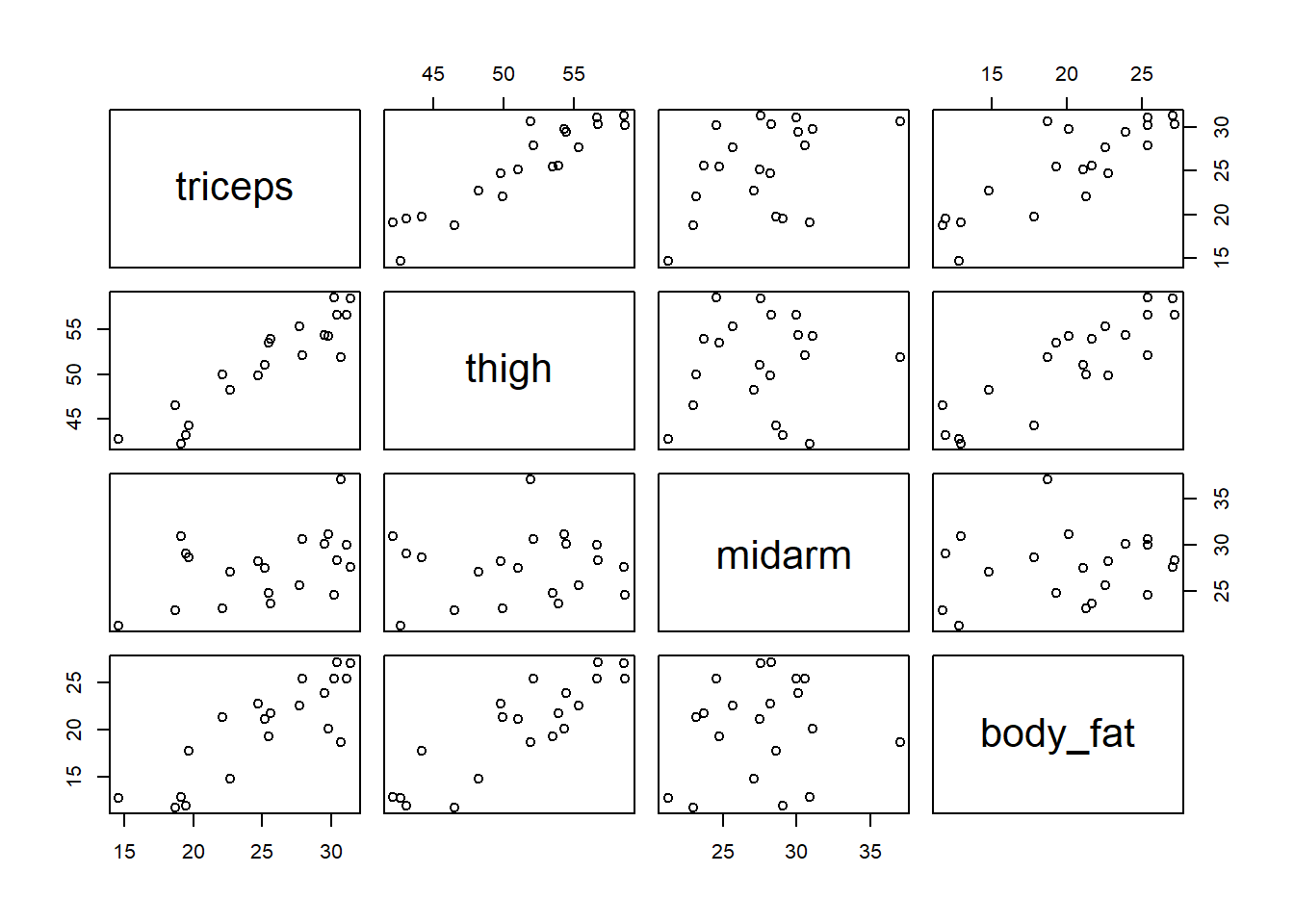
We can use the cor() function to calculate pairwise correlations. Below we round the correlations to two decimal places using the round() function. We see that triceps skinfold and thigh circumference are both highly correlated with our dependent variable, body fat percentage (0.84 and 0.88, respectively). But we also see that those two predictors are highly correlated with each other (0.92).
round(cor(bf), 2)
         triceps thigh midarm body_fat
triceps     1.00  0.92   0.46     0.84
thigh       0.92  1.00   0.08     0.88
midarm      0.46  0.08   1.00     0.14
body_fat    0.84  0.88   0.14     1.00
Let’s model body fat as a function of all three predictors.
m <- lm(body_fat ~ triceps + thigh + midarm, data = bf)
summary(m)
Call:
lm(formula = body_fat ~ triceps + thigh + midarm, data = bf)

Residuals:
    Min      1Q  Median      3Q     Max
-3.7263 -1.6111  0.3923  1.4656  4.1277

Coefficients:
            Estimate Std. Error t value Pr(>|t|)
(Intercept)  117.085     99.782   1.173    0.258
triceps        4.334      3.016   1.437    0.170
thigh         -2.857      2.582  -1.106    0.285
midarm        -2.186      1.595  -1.370    0.190

Residual standard error: 2.48 on 16 degrees of freedom
Multiple R-squared:  0.8014,    Adjusted R-squared:  0.7641
F-statistic: 21.52 on 3 and 16 DF,  p-value: 7.343e-06
The summary shows some weird results. The coefficient for thigh circumference is negative (-2.857) despite the plot above showing a positive association with body fat. But the standard error for thigh circumference is also large (2.582) relative to the coefficient, indicating the estimate is highly variable and uncertain. We also have a relatively large adjusted R-squared (0.76) but no “significant” coefficients. All of these are the telltale signs of multicollinearity.
Let’s check the VIF values of our predictors. We can do that using the vif() function from the car package. This package does not come with R and will need to be installed using install.packages("car") if you don’t have it.
library(car)
vif(m)
 triceps    thigh   midarm
708.8429 564.3434 104.6060
These factors are huge. Recall a VIF value of 10 or higher is the usual threshold for alarm.
It appears multicollinearity is a major problem for this model. How do we address it?
Option 1: Do Nothing
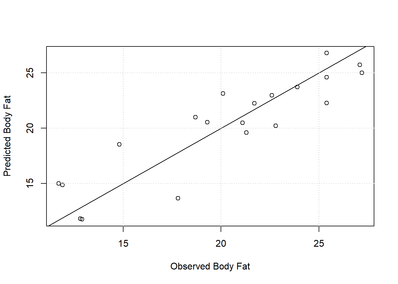
Since the goal of the model is prediction, as opposed to understanding association, it doesn’t really matter how precisely we estimate the coefficients or whether or not they’re “significant”. Our main concern is that the model produces good predictions. Below we create a calibration plot by plotting model predicted body fat versus observed body fat. A good model should produce points that hug the 1:1 diagonal line. Considering we only have 20 observations, the model works fairly well. With a residual standard error of 2.48 reported in the model summary, we expect our model to predict body fat to within about 2-3 percentage points of the real value. The lower accuracy may be an acceptable trade off for the low cost and ease of obtaining the three measurements.
plot(x = bf$body_fat, y = fitted(m),
     xlab = "Observed Body Fat",
     ylab = "Predicted Body Fat")
abline(a = 0, b = 1) # add 1-to-1 diagonal line
grid()
If you’re building a predictive model, multicollinearity is likely not an issue you need to worry about, particularly if it’s safe to assume new data will exhibit the same pattern of multicollinearity and be in the same range of the data used to build the model.
Option 2: Drop Predictors
If you’re interested in quantifying associations in a simple additive model, and you have good reason to believe one of the predictors is redundant (i.e. explains the same information or doesn’t contribute much new information), then you can try dropping the redundant predictor.
Let’s take another look at the correlation matrix for our data.
round(cor(bf), 2)
         triceps thigh midarm body_fat
triceps     1.00  0.92   0.46     0.84
thigh       0.92  1.00   0.08     0.88
midarm      0.46  0.08   1.00     0.14
body_fat    0.84  0.88   0.14     1.00
Triceps skinfold and thigh circumference have a correlation of 0.92. It may be safe to conclude that one of those predictors is redundant. Let’s drop thigh measurement and fit a reduced model.
m2 <- lm(body_fat ~ triceps + midarm, data = bf)
summary(m2)
Call:
lm(formula = body_fat ~ triceps + midarm, data = bf)

Residuals:
    Min      1Q  Median      3Q     Max
-3.8794 -1.9627  0.3811  1.2688  3.8942

Coefficients:
            Estimate Std. Error t value Pr(>|t|)
(Intercept)   6.7916     4.4883   1.513   0.1486
triceps       1.0006     0.1282   7.803 5.12e-07 ***
midarm       -0.4314     0.1766  -2.443   0.0258 *
---
Signif. codes:  0 '***' 0.001 '**' 0.01 '*' 0.05 '.' 0.1 ' ' 1

Residual standard error: 2.496 on 17 degrees of freedom
Multiple R-squared:  0.7862,    Adjusted R-squared:  0.761
F-statistic: 31.25 on 2 and 17 DF,  p-value: 2.022e-06
The summary output shows coefficients that are more precisely estimated. The standard errors are smaller which means we get “significant” results. According to the model, each 1 mm increase in triceps skinfold is associated with about 1 percent increase in body fat, assuming midarm circumference is held constant. Likewise, each 1 cm increase in midarm circumference is associated with a 0.43 decrease in body fat, assuming triceps skinfold is held constant. This latter association seems unusual (bigger arms means less body fat?), but the estimate is small and not very precise. We should be cautious before reading too much into that relationship. In addition, we may want to ask ourselves if it’s realistic to consider varying midarm circumference while holding triceps skinfold thickness fixed, and vice versa. These are two measurements on the same body part. It seems reasonable to assume they would change in tandem. The sample correlation of 0.46 provides some evidence for this.
Checking the VIF for this model seems to indicate we have addressed the multicollinearity. (Notice we get the same VIF for each predictor. That always happens when you calculate VIFs for models with just two predictors. That’s because each predictor’s VIF depends solely on its correlation with the other predictor.)
vif(m2)
 triceps   midarm
1.265118 1.265118
We can also compare this smaller model to the original model using a partial F test since the smaller model is a subset of the larger model (sometimes called a “nested” model). The null of this test is that the two models are no different in their ability to explain the variability in body fat. The large p-value provides evidence in favor of the null hypothesis.
anova(m2, m)
Analysis of Variance Table

Model 1: body_fat ~ triceps + midarm
Model 2: body_fat ~ triceps + thigh + midarm
  Res.Df     RSS Df Sum of Sq      F Pr(>F)
1     17 105.934
2     16  98.405  1    7.5293 1.2242 0.2849
It appears the smaller model is just as effective as the full model. From a practical standpoint, this seems like good news. We only need to take measurements on a female’s arm to estimate body fat. But a drawback of removing variables is that we lose information. In this case thigh circumference and triceps skinfold do not have an exact linear association. With only 20 observations, it may be premature to assume thigh circumference is redundant.
When it comes to dropping variables, another strategy we might consider is removing those variables that appear to have little or no bivariate association with the outcome. In the pairwise scatterplots above, midarm seems to have virtually no relation to body fat, and their correlation is only 0.14. But this type of variable inspection is frowned upon. A variable’s isolated effect on an outcome might change when several variables are considered simultaneously (Sun et al., 1996).
On the other hand, Kutner et al. tell us that midarm is highly correlated with tricep and thigh together. In other words, there is conditional association between the predictors. To investigate, we can regress midarm on tricep and thigh.
mod <- lm(midarm ~ thigh + triceps, data = bf)
summary(mod)
Call:
lm(formula = midarm ~ thigh + triceps, data = bf)

Residuals:
     Min       1Q   Median       3Q      Max
-0.58200 -0.30625  0.02592  0.29526  0.56102

Coefficients:
            Estimate Std. Error t value Pr(>|t|)
(Intercept) 62.33083    1.23934   50.29   <2e-16 ***
thigh       -1.60850    0.04316  -37.26   <2e-16 ***
triceps      1.88089    0.04498   41.82   <2e-16 ***
---
Signif. codes:  0 '***' 0.001 '**' 0.01 '*' 0.05 '.' 0.1 ' ' 1

Residual standard error: 0.377 on 17 degrees of freedom
Multiple R-squared:  0.9904,    Adjusted R-squared:  0.9893
F-statistic: 880.7 on 2 and 17 DF,  p-value: < 2.2e-16
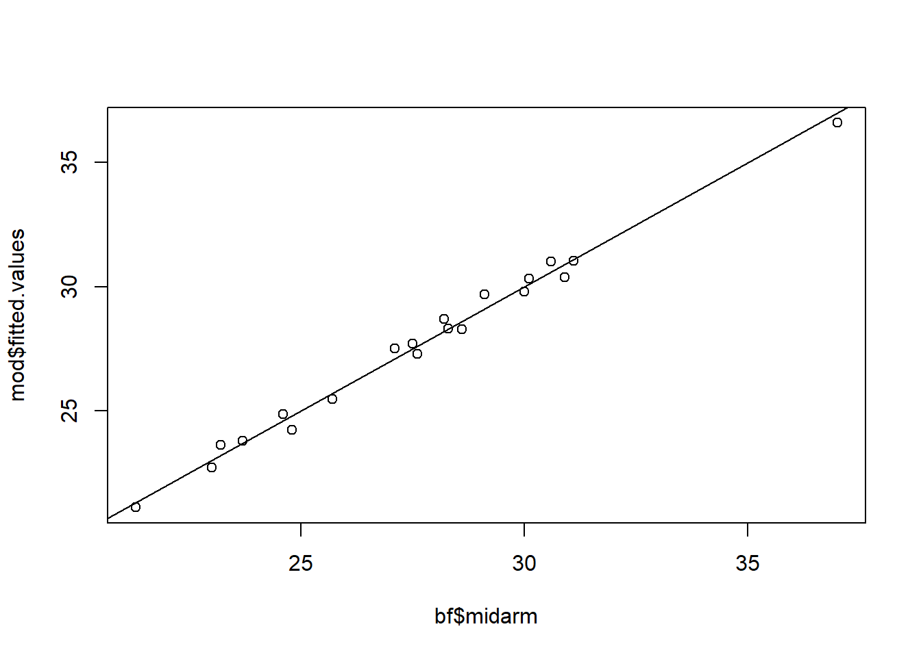
Look at the high R-squared: 0.99. It turns out that midarm circumference can be almost perfectly predicted by thigh circumference and triceps skinfolds. We see this in the calibration plot as well.
plot(bf$midarm, mod$fitted.values)
abline(0, 1)
So perhaps we could be justified in dropping the midarm variable. Let’s try that.
m3 <- lm(body_fat ~ triceps + thigh, data = bf)
summary(m3)
Call:
lm(formula = body_fat ~ triceps + thigh, data = bf)

Residuals:
    Min      1Q  Median      3Q     Max
-3.9469 -1.8807  0.1678  1.3367  4.0147

Coefficients:
            Estimate Std. Error t value Pr(>|t|)
(Intercept) -19.1742     8.3606  -2.293   0.0348 *
triceps       0.2224     0.3034   0.733   0.4737
thigh         0.6594     0.2912   2.265   0.0369 *
---
Signif. codes:  0 '***' 0.001 '**' 0.01 '*' 0.05 '.' 0.1 ' ' 1

Residual standard error: 2.543 on 17 degrees of freedom
Multiple R-squared:  0.7781,    Adjusted R-squared:  0.7519
F-statistic:  29.8 on 2 and 17 DF,  p-value: 2.774e-06
The thigh coefficient is positive and seems to make sense. Every one 1 cm increase in thigh circumference is associated with a 0.66 increase in body fat, holding triceps skinfold constant. But the coefficient for triceps skinfold is much smaller and more uncertain than it was in model m2. Which model is telling the truth about the relationship between triceps skinfold and body fat? And, of course, there’s the issue of whether it even makes sense to interpret these coefficients. Recall that triceps skinfold and thigh circumference have a sample correlation of 0.92. It’s difficult to imagine changing one of these variables while holding the other constant.
Since thigh circumference and triceps skinfold are highly correlated, we might expect large VIF values. But the VIFs are acceptable for model m3.
vif(m3)
 triceps    thigh
6.825239 6.825239
And the model is no worse than the model with all three predictors.
anova(m3, m)
Analysis of Variance Table

Model 1: body_fat ~ triceps + thigh
Model 2: body_fat ~ triceps + thigh + midarm
  Res.Df     RSS Df Sum of Sq      F Pr(>F)
1     17 109.951
2     16  98.405  1    11.546 1.8773 0.1896
Since model m3 does not use a subset of the variables in model m2 (i.e., they are not nested), we cannot compare them using a partial F test. However we can compare them using an information criterion such as AIC. This reveals no appreciable difference between the models.
AIC(m2, m3)
   df      AIC
m2  4 98.09925
m3  4 98.84355
So which model do we prefer? Since the midarm variable appears to be a function of the thigh and triceps variables, model m3 seems like the logical choice. But model m2 might allow us to get a fairly accurate prediction of body fat with only two measurements on someone’s arm. It’s a tough call. In either case, interpreting the coefficients will be problematic since it’s not realistic to imagine these variables being held constant while the other varies.
This leads us to our next option, where we keep all our predictors and employ a different modeling procedure.
Option 3: Ridge Regression
Ridge regression is basically linear modeling with limits on the size of the coefficients. As we saw above, collinear predictors can produce estimated coefficients that are wildly uncertain and unstable. Ridge regression provides a way to keep those coefficient estimates in check by penalizing them and shrinking them closer to 0. The drawback to the penalization is that the coefficients tend to be biased (i.e., wrong). But the bias may be small enough and acceptable if the estimated coefficient is less variable.
The penalization is dictated by a tuning parameter, often symbolized with \(\lambda\) or \(k\). We have to determine this parameter. When \(k = 0\), ridge regression reduces to a standard linear model, also known as ordinary least squares (OLS), which we used in the previous sections. As \(k\) approaches \(\infty\), the effect of the penalty increases and forces the coefficients to 0. Clearly we need to find an optimal value of \(k\). Fortunately there are methods to help us with this task.
We can fit ridge regression models in R using the lmridge package (Imdad et al., 2018). You’ll need to install this package if you don’t already have it using the install.packages() function. Below we specify that we want to model body_fat as a function of all other predictors in the “bf” data frame using the syntax body_dat ~ .. We set the K argument to seq(0, 3, 0.01) which says to try all \(k\) values ranging from 0 to 3 in steps of 0.01. Determining the range of \(k\) sometimes requires a bit of experimentation.
library(lmridge)
ridge.mod <- lmridge(body_fat ~ ., data = bf,
                      K = seq(0, 3, 0.01))
To see the best \(k\) value as determined by generalized cross validation (GCV), we can use the following code:
kest(ridge.mod)$kGCV
[1] 0.07
Running just kest(ridge.mod) will show over 20 estimated values for an optimal \(k\) using different methods proposed over the years. We picked GCV as it seems to be a commonly used metric for selecting \(k\) (James et al. 2021).
To see the coefficients for this model we can run the following code:
coef(ridge.mod)["K=0.07",]
Intercept   triceps     thigh    midarm
 -9.95100   0.44819   0.43618  -0.12726
But it’s probably easier to just a fit a new model using the selected value of \(k\). This allows us to call summary() on the model fit and get additional information about the model.
K <- kest(ridge.mod)$kGCV
ridge.mod <- lmridge(body_fat ~ ., data = bf,
                     K = K)
summary(ridge.mod)
Call:
lmridge.default(formula = body_fat ~ ., data = bf, K = K)


Coefficients: for Ridge parameter K= 0.07
           Estimate Estimate (Sc) StdErr (Sc) t-value (Sc) Pr(>|t|)
Intercept   -9.9510     -681.5229    107.5205      -6.3385   <2e-16 ***
triceps      0.4482        9.8136      1.3394       7.3271   <2e-16 ***
thigh        0.4362        9.9523      1.5944       6.2422   <2e-16 ***
midarm      -0.1273       -2.0230      2.2186      -0.9119   0.3745
---
Signif. codes:  0 '***' 0.001 '**' 0.01 '*' 0.05 '.' 0.1 ' ' 1

Ridge Summary
      R2   adj-R2 DF ridge        F      AIC      BIC
 0.72330  0.69080  1.90771 21.80598 37.75411 99.56832
Ridge minimum MSE= 13965.62 at K= 0.07
P-value for F-test ( 1.90771 , 17.9855 ) = 1.865521e-05
-------------------------------------------------------------------
The first column, Estimate, contains the ridge regression coefficients. Notice they’ve all been shrunk toward 0 and are smaller than the original coefficients in the linear model. The other columns with “(Sc)” appended are for the scaled versions of the coefficients. See The R Journal article about the lmridge package for more information on the summary output.
We can visually assess the performance of the ridge regression model with a calibration plot. Below we generate calibration plots for the linear model and ridge regression model, both of which use all three predictors.
op <- par(mfrow = c(1,2))
plot(x = bf$body_fat, y = fitted(m),
     xlab = "Observed Body Fat",
     ylab = "Predicted Body Fat",
     main = "Linear Model (OLS)")
abline(a = 0, b = 1) # add 1-to-1 diagonal line
grid()
plot(x = bf$body_fat, y = predict(ridge.mod),
     xlab = "Observed Body Fat",
     ylab = "Predicted Body Fat",
     main = "Ridge Regression")
abline(a = 0, b = 1) # add 1-to-1 diagonal line
grid()

par(op)
It’s difficult to judge by eye which model is better from a predictive standpoint. A more objective way to determine this is using Mean Square Error (MSE). This is simply the mean of the squared residuals. The smaller the mean, the better the fit.
c("OLS" = mean(residuals(m)^2),
  "Ridge" = mean(residuals(ridge.mod)^2))
     OLS    Ridge
4.920244 5.457193
The linear OLS model seems better based on this metric. But the MSE values were calculated on the same data used to build the models. They’re almost certainly too optimistic. The ridge model might perform better on new data. We don’t have new data but we can use cross validation to estimate the MSE for new data. Since we only have 20 observations, we can use leave-one-out (LOO) cross validation (CV). This means we build 20 models using only 19 observations and then test the model on the held out observation. We do this such that each observation gets a turn at being held out for testing.
First we perform LOO CV for the original linear model. Notice the MSE almost doubles.
lm_pred <- numeric(20)
for(i in 1:20){
    m <- lm(body_fat ~ ., data = bf[-i,])
    lm_pred[i] <- predict(m, newdata = bf[i,])
}

# calculate MSE
mean((bf$body_fat - lm_pred)^2)
[1] 8.036828
Now we perform LOO CV for the ridge regression model. Notice we need to estimate an optimal tuning parameter each time. The MSE is now even larger than the linear model.
ridge_pred <- numeric(20)
for(i in 1:20){
    ridge.mod <- lmridge(body_fat ~ ., data = bf[-i,], K = seq(0, 3, 0.01))
    K <- kest(ridge.mod)$kGCV
    ridge.mod <- lmridge(body_fat ~ ., data = bf[-i,], K = K)
    ridge_pred[i] <- predict(ridge.mod, newdata = bf[i,])
}

# calculate MSE
mean((bf$body_fat - ridge_pred)^2)
[1] 9.261193
It looks like the linear model may be the better predictive model in this case. But if the goal of the model is to assign meaning to the coefficients, we may prefer the ridge regression estimates since they’re more stable. Again, though, the usual interpretation of model coefficients may not be practical in the presence of collinear predictors. For more details on Ridge Regression, we recommend Chapter 6 (section 6.2) of An Introduction to Statistical Learning (James et al. 2021).
Option 4: Principal Components
If you have many variables that exhibit multicollinearity, it might makes sense to transform those variables into principal components. This is often called a principal component analysis (PCA). Principal components are linear combinations of data that can be used to represent that same data in fewer dimensions. For example, 15 variables might be reduced to two principal components that explain most of the variation in the data. We could then fit a model using the two principal components as predictors instead of all 15 variables.
With only three predictors, our body fat data is not an ideal candidate for PCA. However we can still use the data to demonstrate the method. One approach is to use the prcomp() function that comes with R. The first argument takes a data frame (or matrix) that contains the variables you want to transform. An optional second argument is “scale.”, which allows you to indicate whether or not you want to scale the variables to have unit variance. This is usually advisable. (By default, prcomp() centers all variables to have mean 0.) Calling summary() on the saved object returns a summary of the amount of variation explained by the principal components.
bf_pca <- prcomp(bf[,1:3], scale. = TRUE)
summary(bf_pca)
Importance of components:
                          PC1    PC2     PC3
Standard deviation     1.4375 0.9658 0.02696
Proportion of Variance 0.6888 0.3109 0.00024
Cumulative Proportion  0.6888 0.9998 1.00000
We see the first component (PC1) explains about 69% of the variation in the data. The second component (PC2) explains about 31% of the variation. Together these two components explain almost all of the variation in the data.
The rotation matrix contains the loadings of the variables, which are the weights used to derive the principal components.
bf_pca$rotation
              PC1         PC2        PC3
triceps 0.6946957 -0.05010563  0.7175565
thigh   0.6294279 -0.44050902 -0.6401347
midarm  0.3481645  0.89634883 -0.2744818
Let’s see how loadings are used to calculate principal components. We’ll demonstrate how to calculate the first principal component for our first observation. To begin, get the data for the first subject.
bf[1, 1:3]
  triceps thigh midarm
1    19.5  43.1   29.1
But recall we had prcomp() center and scale each variable to have mean 0 and variance 1 when we ran it, so we need to do the same. We can do that with the scale() function. Notice we scale first, and then subset to get the first row.
scale(bf[,1:3])[1,]
   triceps      thigh     midarm
-1.1556243 -1.5416617  0.4057966
To calculate PC1, we multiply each data value by its corresponding loading and take the sum. This is a linear combination of the data.
-1.155624*0.6946957 + -1.541662*0.6294279 + 0.4057966*0.3481645
[1] -1.631888
This is the first principal component for observation 1. You’ll be happy to know that the prcomp() function calculates this for us. It’s located in the “x” element of the saved object. Notice it also calculates PC2 and PC3. Below we just show the principal components for the first observation. These are sometimes referred to as scores.
bf_pca$x[1, ]
        PC1         PC2         PC3
-1.63188801  1.10075447  0.04626157
Principal components are calculated such that they are completely uncorrelated with one another. The term for this is orthogonal. We can see this by calculating the correlation matrix for the principal components. Notice the correlations between components are all 0.
round(cor(bf_pca$x), 3)
    PC1 PC2 PC3
PC1   1   0   0
PC2   0   1   0
PC3   0   0   1
If we like, we can use the principal components as predictors in a regression model. Since they’re orthogonal, there is no risk of collinearity. Ideally, we would only use the first few components assuming they explain most of the variation in the data. Let’s try using the first and second principal components to predict body fat since they explain over 99% of the variation.
m4 <- lm(bf$body_fat ~ bf_pca$x[,1:2])
summary(m4)
Call:
lm(formula = bf$body_fat ~ bf_pca$x[, 1:2])

Residuals:
    Min      1Q  Median      3Q     Max
-3.9862 -1.8853  0.2665  1.3179  4.0244

Coefficients:
                   Estimate Std. Error t value Pr(>|t|)
(Intercept)         20.1950     0.5656  35.707  < 2e-16 ***
bf_pca$x[, 1:2]PC1   2.9358     0.4037   7.273  1.3e-06 ***
bf_pca$x[, 1:2]PC2  -1.6498     0.6008  -2.746   0.0138 *
---
Signif. codes:  0 '***' 0.001 '**' 0.01 '*' 0.05 '.' 0.1 ' ' 1

Residual standard error: 2.529 on 17 degrees of freedom
Multiple R-squared:  0.7805,    Adjusted R-squared:  0.7546
F-statistic: 30.22 on 2 and 17 DF,  p-value: 2.528e-06
The estimated coefficients are large and significant. That seems promising. Unfortunately, it’s challenging to interpret what PC1 and PC2 represent. Also, despite only using two predictors in the model, we still need all three original variables to calculate the principal components. Nevertheless, PCA can sometimes be an effective method for dealing with many highly correlated values. There are more steps and considerations for PCA than we have covered in this article. For more details, we recommend Chapter 6 (section 6.3) of An Introduction to Statistical Learning (James et al. 2021).
Simulated models with correlated predictors
We reviewed four options for dealing with multicollinearity: do nothing, drop variables, ridge regression, and PCA. There are certainly other options, including Bayesian modeling with strong priors, the Elastic Net method, and Full-Subsets Multiple Regression, but the four presented are probably the most common approaches. Which option you choose depends on the goal of the model and the severity of the collinearity. Now let’s investigate multicollinearity using simulated data. What happens when we generate an outcome using data that is collinear?
Below we use the mvrnorm() function from the MASS package to generate 300 observations of three predictors, all with mean 0, standard deviation 1, and a high correlation of 0.99. Then we generate an outcome using a simple additive model of those correlated predictors with coefficients arbitrarily set to 0.5, -0.5, and 0.9. We also add some noise to the outcome by sampling from a Normal distribution with mean 0 and standard deviation 0.3.
library(MASS)
set.seed(20)
n <- 300
r <- 0.99
d <- as.data.frame(mvrnorm(n = n, mu = c(0,0,0),
             Sigma = matrix(c(1,r,r,
                              r,1,r,
                              r,r,1),
                            byrow = T,
                            nrow = 3)))
d$Y <- 0.2 + 0.5*d$V1 + -0.5*d$V2 + 0.9*d$V3 +
  rnorm(n = n, sd = 0.3)
We can see the predictors are indeed highly correlated.
cor(d)
          V1        V2        V3         Y
V1 1.0000000 0.9896087 0.9902453 0.9513259
V2 0.9896087 1.0000000 0.9896350 0.9377561
V3 0.9902453 0.9896350 1.0000000 0.9537596
Y  0.9513259 0.9377561 0.9537596 1.0000000
Now we fit a model using all three correlated predictors and check the summary. Notice we’re fitting the “true” model. The proposed model is the model used to simulate the data. The estimated coefficients and standard errors look fine.
m <- lm(Y ~ V1 + V2 + V3, data = d)
summary(m)
Call:
lm(formula = Y ~ V1 + V2 + V3, data = d)

Residuals:
     Min       1Q   Median       3Q      Max
-0.64289 -0.18245  0.02629  0.17418  0.75999

Coefficients:
            Estimate Std. Error t value Pr(>|t|)
(Intercept)  0.17172    0.01607  10.683  < 2e-16 ***
V1           0.61767    0.12926   4.778 2.79e-06 ***
V2          -0.57011    0.12556  -4.540 8.18e-06 ***
V3           0.85323    0.12906   6.611 1.78e-10 ***
---
Signif. codes:  0 '***' 0.001 '**' 0.01 '*' 0.05 '.' 0.1 ' ' 1

Residual standard error: 0.2771 on 296 degrees of freedom
Multiple R-squared:  0.9178,    Adjusted R-squared:  0.917
F-statistic:  1102 on 3 and 296 DF,  p-value: < 2.2e-16
The 95% confidence intervals of the coefficient estimates all capture the true values used to generate the data.
cbind(confint(m)[2:4,], "True Values" = c(0.5, -0.5, 0.9))
        2.5 %     97.5 % True Values
V1  0.3632854  0.8720615         0.5
V2 -0.8172242 -0.3229983        -0.5
V3  0.5992263  1.1072243         0.9
Looking at VIFs might make us reconsider our model. They’re much greater than 10.
car::vif(m)
      V1       V2       V3
67.02465 63.09730 67.19383
But we know we fit the correct model, and our estimates are reasonable and fairly precise. We have no reason to change the model. The VIFs are correct that we have multicollinearity, but they don’t measure model performance. Having VIFs less than 10 does not mean we have a good model, and having VIFs greater than 10 does not mean we have a bad model.
Of course we just simulated one data set using a seed. What happens if we try this many times? Below we replicate what we just did 1000 times and summarize the distributions of the coefficients and their standard errors.
rout <- replicate(n = 1000, expr = {
                  d <- as.data.frame(mvrnorm(n = n, mu = c(0,0,0),
                                             Sigma = matrix(c(1,r,r,
                                                              r,1,r,
                                                              r,r,1),
                                                            byrow = T,
                                                            nrow = 3)))
                  d$Y <- 0.2 + 0.5*d$V1 + -0.5*d$V2 + 0.9*d$V3 +
                    rnorm(n = n, sd = 0.3)
                  m <- lm(Y ~ ., data = d)
                  # extract coefficients and their SEs
                  c(coef(m)[-1], coef(summary(m))[-1,2])})
rownames(rout) <- c("V1", "V2", "V3", "V1 SE", "V2 SE", "V3 SE")
apply(rout, 1, summary)
               V1          V2        V3     V1 SE     V2 SE     V3 SE
Min.    0.1167174 -1.04914851 0.4731471 0.1173488 0.1206018 0.1162677
1st Qu. 0.4000896 -0.59080884 0.8041736 0.1372277 0.1364114 0.1371338
Median  0.5011103 -0.49355189 0.9002364 0.1421406 0.1417376 0.1420293
Mean    0.4998070 -0.49957104 0.8999321 0.1425915 0.1421041 0.1424768
3rd Qu. 0.5967001 -0.40289622 0.9917656 0.1478256 0.1470749 0.1475023
Max.    1.0451780 -0.09674094 1.3272648 0.1684968 0.1846908 0.1649418
The distribution of coefficients and their standard errors have a reasonable range despite the severe multicollinearity. All coefficients consistently have the correct sign and all standard errors are stable with a range of about 0.5.
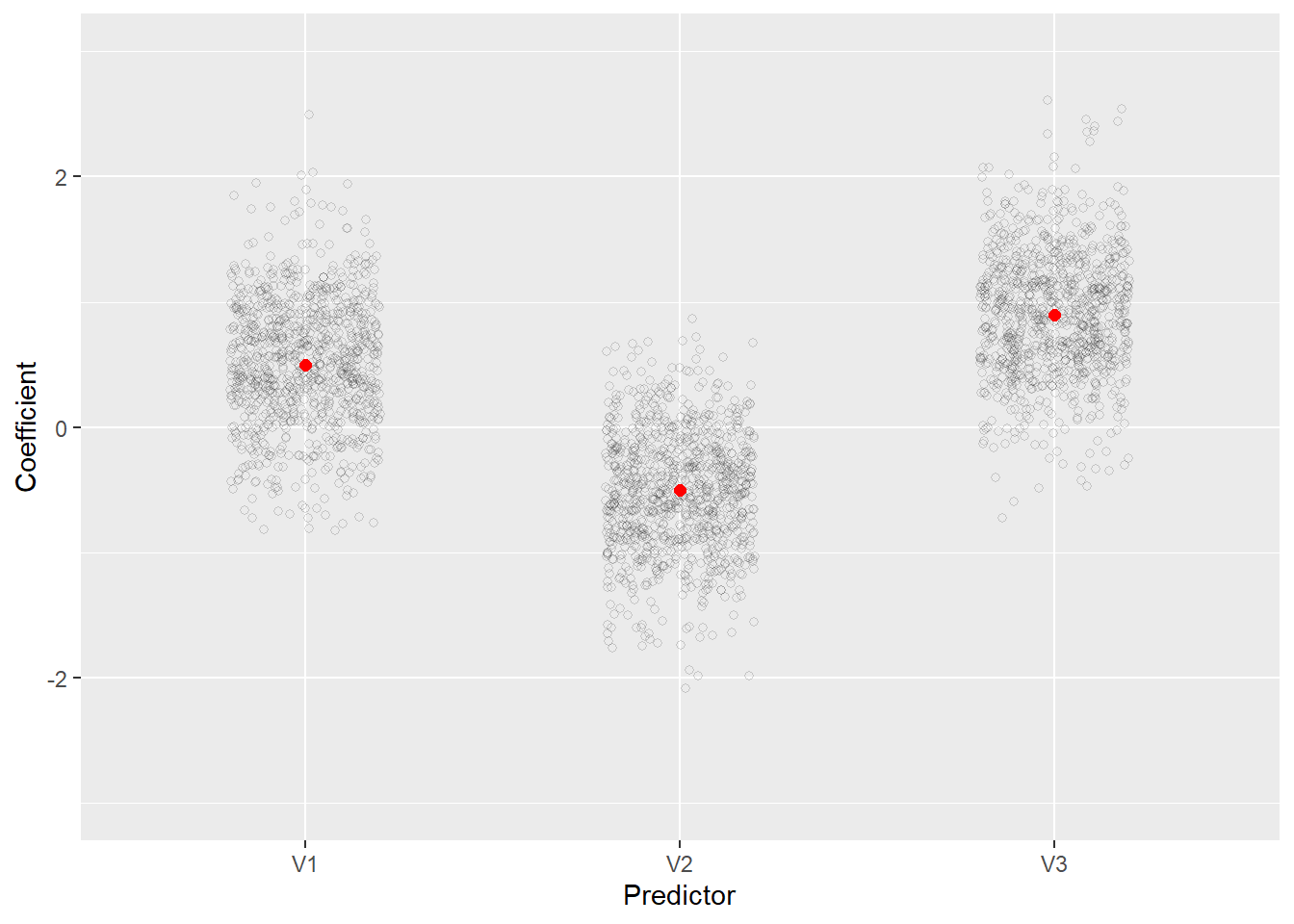
We can also plot the coefficients. Below we use the tidyr and ggplot2 packages to prepare the data and create the plot, respectively. Notice how they cluster around the true values (the red dots). We see that when we fit the correct model, the estimated coefficients are reasonable and unbiased even though the predictors are highly correlated.
library(tidyr)
library(ggplot2)

# select the first three rows, transpose, and reshape the data to "long" format
rout_df <- t(rout[1:3,]) |>
  as.data.frame() |>
  pivot_longer(cols = everything(),
               names_to = "Predictor",
               values_to = "Coefficient")

ggplot(rout_df) +
  aes(x = Predictor, y = Coefficient) +
  geom_jitter(width = 0.2, height = 0, alpha = 1/6, shape = 1) +
  annotate(geom = "point", x = 1:3, y = c(0.5, -0.5, 0.9),
           color = "red", size = 2) +
  scale_y_continuous(limits = c(-3,3))

What if we reduce the sample size from 300 to 30?
n <- 30 # reducing the sample size
rout <- replicate(n = 1000, expr = {
                  d <- as.data.frame(mvrnorm(n = n, mu = c(0,0,0),
                                             Sigma = matrix(c(1,r,r,
                                                              r,1,r,
                                                              r,r,1),
                                                            byrow = T,
                                                            nrow = 3)))
                  d$Y <- 0.2 + 0.5*d$V1 + -0.5*d$V2 + 0.9*d$V3 +
                    rnorm(n = n, sd = 0.3)
                  m <- lm(Y ~ ., data = d)
                  # extract coefficients and their SEs
                  c(coef(m)[-1], coef(summary(m))[-1,2])})
rownames(rout) <- c("V1", "V2", "V3", "V1 SE", "V2 SE", "V3 SE")
apply(rout, 1, summary)
                V1         V2         V3     V1 SE     V2 SE     V3 SE
Min.    -0.8218766 -2.0800567 -0.7239886 0.2720820 0.2661198 0.2655169
1st Qu.  0.1933113 -0.8481240  0.5633730 0.4138150 0.4126413 0.4078599
Median   0.5216105 -0.5266352  0.9047253 0.4698390 0.4684414 0.4661539
Mean     0.5166280 -0.5215176  0.9016317 0.4787598 0.4771618 0.4749131
3rd Qu.  0.8680898 -0.1941328  1.2179005 0.5341907 0.5331722 0.5293820
Max.     2.4908720  0.8647349  2.6133107 0.8477958 0.8765595 0.8304091
Now we begin to see more fluctuation in the estimates. Clearly smaller sample sizes combined with multicollinearity can lead to greater uncertainty in estimating model coefficients, even when we’re fitting the correct model. The plot also shows the increased uncertainty in the estimated coefficients.
rout_df <- t(rout[1:3,]) |>
  as.data.frame() |>
  pivot_longer(cols = everything(),
               names_to = "Predictor",
               values_to = "Coefficient")

ggplot(rout_df) +
  aes(x = Predictor, y = Coefficient) +
  geom_jitter(width = 0.2, height = 0, alpha = 1/6, shape = 1) +
  annotate(geom = "point", x = 1:3, y = c(0.5, -0.5, 0.9),
           color = "red", size = 2) +
  scale_y_continuous(limits = c(-3,3))
Conclusion
Multicollinearity is tricky and not something you can address just by looking at pairwise correlations and VIFs. How you handle it depends on your goal.
- If you’re building a model to make predictions, it’s probably something you can safely disregard, or at least rank lower on your list of concerns about model building.
- If you’re building a model for understanding associations, it’s not always clear what to do about multicollinearity. If you have truly redundant variables, where correlation is 1, then it’s advisable to drop one of those variables. But just because you have “high” correlation between variables (say around 0.8 or 0.9) does not necessarily mean one of the variables should be removed. It’s possible both variables play a significant role in explaining the outcome.
- Ridge regression is a common method for dealing with multicollinearity, but still requires specifying a correct model. You can’t just plug in all your predictors in a single additive model and expect it to be correct. You still need to use subject matter knowledge when specifying a model, and that may mean adding interactions and/or non-linear effects.
- VIFs are good at detecting multicollinearity, but they don’t tell you how to address it. Low VIFs suggest the standard errors of your coefficients are not inflated due to collinearity, but they don’t mean you have a good model. High VIFs suggest you have multicollinearity, but they don’t mean you have a bad model.
- Interpreting coefficients in the presence of multicollinearity should be carried out with caution. Holding one variable constant while the other varies may not be realistic if the variables are highly correlated.
R session details
The analysis was done using the R Statistical language (v4.5.1; R Core Team, 2025) on Windows 11 x64, using the packages car (v3.1.3), carData (v3.0.5), lmridge (v1.2.2), MASS (v7.3.65), ggplot2 (v3.5.2) and tidyr (v1.3.1).
References
- Faraway J. (2025). Linear Models with R, 3rd Ed. CRC Press.
- Fox J & Weisberg S. (2019). An R Companion to Applied Regression, Third edition. Sage, Thousand Oaks CA. https://www.john-fox.ca/Companion/.
- Graham, M.H. (2003), CONFRONTING MULTICOLLINEARITY IN ECOLOGICAL MULTIPLE REGRESSION. Ecology, 84: 2809-2815. https://doi.org/10.1890/02-3114.
- Imdad, MU & Aslam M. (2018). lmridge: Linear Ridge Regression with Ridge Penalty and Ridge Statistics. R package version 1.2.2, https://CRAN.R-project.org/package=lmridge.
- Imdad, MU, Aslam M, and Altaf S. (2018). “lmridge: A Comprehensive R Package for Ridge Regression.” The R Journal 10 (2): 326-346. https://doi.org/10.32614/RJ-2018-060.
- James G, Witten D, Hastie T, and Tibshirani R. (2021) Introduction to Statistical Learning, Second Edition. Springer. https://www.statlearning.com/.
- Kutner MH, Nachtsheim, CJ, Neter J, and Li W. (2005). Applied Linear Statistical Models, 5th Ed.. McGraw Hill.
- Lumley, T. (2024, November 21). Collinearity four more times. Biased and Inefficient. https://notstatschat.rbind.io/2024/11/21/collinearity-again/.
- McElreath, R. (2020). Statistical Rethinking, 2nd Ed. CRC Press.
- R Core Team (2025). R: A Language and Environment for Statistical Computing. R Foundation for Statistical Computing, Vienna, Austria. https://www.R-project.org/.
- Sun GW, Shook TL, Kay GL. Inappropriate use of bivariable analysis to screen risk factors for use in multivariable analysis. Journal of Clinical Epidemiology. 1996. 49, 8:907-16.
- Wickham, H, Vaughan, D, and Girlich, M (2024). tidyr: Tidy Messy Data. https://doi.org/10.32614/CRAN.package.tidyr, R package version 1.3.1, https://CRAN.R-project.org/package=tidyr.
- Wickham, H. (2016). ggplot2: Elegant Graphics for Data Analysis. Springer-Verlag, New York. R package version 3.5.2., https://CRAN.R-project.org/package=ggplot2.
- Zuur, A.F., Ieno, E.N. and Elphick, C.S. (2010), A protocol for data exploration to avoid common statistical problems. Methods in Ecology and Evolution, 1: 3-14. https://doi.org/10.1111/j.2041-210X.2009.00001.x
Clay Ford
Statistical Research Consultant
University of Virginia Library
September 2, 2025
For questions or clarifications regarding this article, contact statlab@virginia.edu.
View the entire collection of UVA Library StatLab articles, or learn how to cite.