Bootstrapped Stepwise Model Selection

Simulate data

Before we get started let’s simulate data we’ll use in the examples that follow. Below we simulate 500 observations consisting of 8 predictor variables (x1 - x8) and a single outcome (y). The predictors consist of randomly generated uniform, normal and exponential variables along with two categorical variables. We generate the outcome, y, using only odd-numbered predictor variables. We also include two interactions between x1 and x3, and x1 and x7. The line of code that generates y is our “true” model. The reason we only use odd-numbered predictor variables is to simulate a real-life setting where only some of the variables in a data set are associated with the outcome. Hopefully the automated selection methods will be able to determine which variables we used to generate the outcome. When finished, we place all the predictors and the outcome in a data frame named “d”. We use the mget() function to grab all the predictors out of the global environment by their character name.

The code set.seed(8989) allows you to generate the same random data if you wish to run this code yourself. (Be sure to run the entire code chunk at one time.)

set.seed(8989)
n <- 500
x1 <- runif(n, 0, 10)
x2 <- runif(n, 0, 10)
x3 <- rnorm(n)
x4 <- x3 + rnorm(n, sd = 0.2)
x5 <- log(rexp(n, rate = 0.01))
x6 <- rexp(n, rate = 0.1)
x7 <- factor(sample(c("M","F"), size = n, replace = TRUE))
x8 <- factor(sample(c("A","B","C","D"), size = n, replace = TRUE))

# generate response; this is the true model
y <- 20 + 1.5*x1 + -0.9*x3 + 1.5*x5 + 1.9*(x7=="M") +
  1.2*x1*x3 + -1.8*x1*(x7=="M") +
  rnorm(n, sd = 2)  # normally distributed residuals with constant variance

# put everything in a data frame
d <- data.frame(y, mget(paste0("x",1:8)))

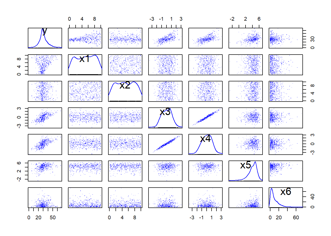
With our data generated, let’s look at pairwise scatter plots of the outcome and numeric predictors. The scatterplotMatrix() function from the car package (Fox and Weisberg, 2019) makes this easy to do. If you don’t have this package, or any other package we use in this article, you can install it using the install.packages() function. The top row visualizes the association of y with each predictor independently. We see the variability of y increases as x1 increases. We also see that x3 and x4 are highly correlated. The diagonals show the distributions of each variable. Our outcome, y, looks mostly symmetric and positive.

# install.packages("car")
library(car)
scatterplotMatrix(d[,1:7], pch = ".", regLine = FALSE, smooth = FALSE)

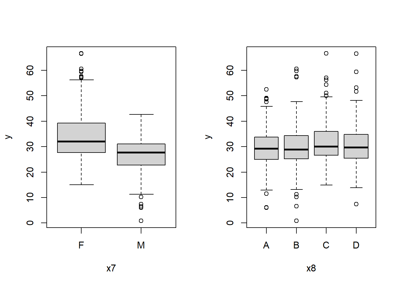
The association of y with the categorical predictors can be investigated with boxplots. In the left plot below we see a slight difference in the median of y between the F and M levels of variable x7. In the right plot we see little difference in y between the levels of x8. In both plots we see constant variability between the levels. We also see a handful of “outliers”, values that lie beyond the extremes of the boxplot “whiskers”. Points that lie beyond 1.5 times the interquartile range from the box are considered outliers. These values may or may not be cause for concern. Subject matter expertise is just as important as a statistical algorithm for determining whether a value is truly an outlier.

op <- par(mfrow = c(1,2))
boxplot(y ~ x7, data = d)
boxplot(y ~ x8, data = d)

Manual model building

Let’s pretend our data is not simulated and that we’re interested in developing a predictive model for y. That is, we would like to create a linear model that we could use to predict future values of y. We’re interested in a linear model so we can understand how our model works and possibly critique it. To begin, we could fit a model including all eight predictors. This is called a main effects model. The model syntax y ~ . says to regress y on all the other variables in the data frame. The variables are entered into the model in the same order they’re stored in the columns of the data frame.

m1 <- lm(y ~ ., data = d)

To assess each predictor’s contribution to the model we’ll use the Anova() function from the car package. This presents a series of tests where each predictor is dropped from the model containing all other predictors. The null hypothesis in each test is that the variable does not help explain variability in the outcome, y. A large F value and small p-value provide evidence against the null. Below we see the odd-numbered variables all appear to explain a substantial amount of variability in the model. Therefore it seems like we should retain those four variables.

Anova(m1)

Anova Table (Type II tests)

Response: y
           Sum Sq  Df  F value    Pr(>F)    
x1         1997.6   1  73.6061 < 2.2e-16 ***
x2           19.7   1   0.7268    0.3943    
x3          639.1   1  23.5492  1.64e-06 ***
x4            1.5   1   0.0539    0.8166    
x5         2263.9   1  83.4177 < 2.2e-16 ***
x6            9.8   1   0.3629    0.5472    
x7         6397.8   1 235.7423 < 2.2e-16 ***
x8           43.0   3   0.5279    0.6633    
Residuals 13271.0 489                       
---
Signif. codes:  0 '***' 0.001 '**' 0.01 '*' 0.05 '.' 0.1 ' ' 1

Now let’s fit a model with all main effects and all 28 two-way interactions. The model syntax y ~ .^2 fits such a model.

m2 <- lm(y ~ .^2, data = d)
Anova(m2)

Anova Table (Type II tests)

Response: y
          Sum Sq  Df   F value  Pr(>F)    
x1        1603.8   1  442.7663 < 2e-16 ***
x2           0.1   1    0.0188 0.89098    
x3         584.2   1  161.2915 < 2e-16 ***
x4           1.2   1    0.3347 0.56321    
x5        2241.0   1  618.6827 < 2e-16 ***
x6           3.0   1    0.8395 0.36003    
x7        5679.5   1 1567.9617 < 2e-16 ***
x8           0.0   3    0.0035 0.99971    
x1:x2        4.6   1    1.2720 0.25999    
x1:x3      364.7   1  100.6800 < 2e-16 ***
x1:x4        7.4   1    2.0559 0.15231    
x1:x5        1.6   1    0.4301 0.51229    
x1:x6        1.3   1    0.3501 0.55434    
x1:x7     3085.7   1  851.8725 < 2e-16 ***
x1:x8       30.8   3    2.8331 0.03793 *  
x2:x3        0.6   1    0.1572 0.69194    
x2:x4        0.3   1    0.0750 0.78434    
x2:x5       15.1   1    4.1726 0.04167 *  
x2:x6        1.1   1    0.3057 0.58060    
x2:x7        1.0   1    0.2832 0.59486    
x2:x8        5.3   3    0.4835 0.69389    
x3:x4       11.9   1    3.2924 0.07027 .  
x3:x5       15.0   1    4.1303 0.04271 *  
x3:x6        3.6   1    0.9832 0.32194    
x3:x7        2.2   1    0.6158 0.43303    
x3:x8        5.3   3    0.4908 0.68884    
x4:x5       15.5   1    4.2895 0.03892 *  
x4:x6        5.2   1    1.4375 0.23119    
x4:x7        4.1   1    1.1293 0.28849    
x4:x8        7.4   3    0.6851 0.56148    
x5:x6        4.9   1    1.3616 0.24388    
x5:x7       19.9   1    5.4983 0.01947 *  
x5:x8       11.6   3    1.0640 0.36407    
x6:x7        0.0   1    0.0000 0.99662    
x6:x8        2.1   3    0.1950 0.89977    
x7:x8       27.5   3    2.5282 0.05681 .  
Residuals 1619.1 447                      
---
Signif. codes:  0 '***' 0.001 '**' 0.01 '*' 0.05 '.' 0.1 ' ' 1

There are several two-way interactions that may be worth keeping. The two most important ones in terms of their F values and p-values are the interactions we defined when simulating the data: x1:x3 and x1:x7. But what about x2:x5? Our main effects model didn’t select x2 as a predictor. But maybe we need it if there’s evidence of it interacting with x5.

To see if we need to keep the interaction of x2 and x5, we could compare models using Akaike’s Information Criterion (AIC). AIC is a model selection criterion we seek to minimize. Between two or more candidate models for the same outcome, we prefer the model with the smallest AIC value. AIC is a powerful model selection criterion because it balances fit and complexity. This means it both rewards models for how well they fit the data and penalizes models with more parameters (i.e., more coefficients). In the eyes of AIC, a more complicated model that provides a marginal improvement in fit will not be preferred to a simpler model that fits almost as well.

Below we use the update() function to update the formula of model m2 to remove the x2:x5 interaction. The syntax . ~ . - x2:x5 means keep the same outcome on the left-hand side and keep all predictors on the right-hand side except x2:x5. Then we compare models using the AIC() function.

m2b <- update(m2, . ~ . - x2:x5)
AIC(m2, m2b)

    df      AIC
m2  54 2114.456
m2b 53 2117.101

The lower AIC of the model with the x2:x5 interaction suggests that we should keep the interaction. But what about the other interactions potentially of interest? Clearly it would be onerous to carry out similar comparisons for each interaction. Plus an interaction’s effect on the outcome might be different in the presence of other interactions.

Automated model selection

Instead of manually fitting different models, we could try using an automated process to select the best model. One approach is using a stepwise algorithm via AIC.¹ The stepAIC() function in the MASS package (included with R) automates this process. But as we’ll see, the final model this process selects depends on the direction you run the algorithm.

Let’s try it out on our m2 model that includes all main effects and two-way interactions. The function produces a lot of output by default, which we don’t want to display in this article, so we set trace = FALSE to suppress it. After running stepAIC(), we use the Anova() function to see what terms were selected.

library(MASS)
m3 <- stepAIC(m2, trace = FALSE)
Anova(m3)

Anova Table (Type II tests)

Response: y
          Sum Sq  Df   F value    Pr(>F)    
x1        1921.9   1  543.5743 < 2.2e-16 ***
x2           0.3   1    0.0708  0.790287    
x3         780.8   1  220.8318 < 2.2e-16 ***
x4           1.6   1    0.4541  0.500704    
x5        2399.9   1  678.7770 < 2.2e-16 ***
x6           3.1   1    0.8658  0.352595    
x7        6015.1   1 1701.2838 < 2.2e-16 ***
x8           0.0   3    0.0040  0.999654    
x1:x3     7513.3   1 2125.0202 < 2.2e-16 ***
x1:x7     3294.5   1  931.7891 < 2.2e-16 ***
x1:x8       33.7   3    3.1802  0.023807 *  
x2:x5       12.1   1    3.4290  0.064684 .  
x3:x4       15.5   1    4.3738  0.037027 *  
x3:x5       20.3   1    5.7474  0.016899 *  
x4:x5       20.1   1    5.6837  0.017516 *  
x4:x6        9.8   1    2.7699  0.096715 .  
x4:x7        8.7   1    2.4548  0.117833    
x5:x7       26.5   1    7.5039  0.006389 ** 
x7:x8       23.3   3    2.1978  0.087529 .  
Residuals 1675.9 474                        
---
Signif. codes:  0 '***' 0.001 '**' 0.01 '*' 0.05 '.' 0.1 ' ' 1

We can see the stepwise algorithm retained 11 of the original 28 interactions, though we know the true model only had two interactions. How did the algorithm arrive at this final model? The anova component of the m3 object shows the path taken.

m3$anova

Stepwise Model Path 
Analysis of Deviance Table

Initial Model:
y ~ (x1 + x2 + x3 + x4 + x5 + x6 + x7 + x8)^2

Final Model:
y ~ x1 + x2 + x3 + x4 + x5 + x6 + x7 + x8 + x1:x3 + x1:x7 + x1:x8 + 
    x2:x5 + x3:x4 + x3:x5 + x4:x5 + x4:x6 + x4:x7 + x5:x7 + x7:x8

      Step Df    Deviance Resid. Df Resid. Dev      AIC
1                               447   1619.127 693.5170
2  - x6:x8  3  2.11936121       450   1621.246 688.1710
3  - x2:x8  3  5.39692337       453   1626.643 683.8327
4  - x3:x8  3  5.38899790       456   1632.032 679.4865
5  - x4:x8  3  6.37803307       459   1638.410 675.4367
6  - x2:x4  1  0.03072998       460   1638.441 673.4460
7  - x6:x7  1  0.10364316       461   1638.544 671.4777
8  - x5:x8  3 13.38931213       464   1651.934 669.5468
9  - x1:x6  1  0.39026401       465   1652.324 667.6649
10 - x2:x6  1  0.88866075       466   1653.212 665.9338
11 - x2:x7  1  1.34336899       467   1654.556 664.3399
12 - x1:x5  1  1.47981318       468   1656.036 662.7869
13 - x3:x7  1  1.78375243       469   1657.819 661.3251
14 - x1:x2  1  2.30966337       470   1660.129 660.0213
15 - x2:x3  1  2.52516678       471   1662.654 658.7812
16 - x5:x6  1  3.29909293       472   1665.953 657.7723
17 - x3:x6  1  3.85010004       473   1669.803 656.9265
18 - x1:x4  1  6.07992746       474   1675.883 656.7438

The first line shows the AIC of the initial model with all main effects and all 28 two-way interactions: 693.5170.² The second line shows that the algorithm first removed the x6:x8 interaction, which reduced the AIC to 688.1710. Next, it removed the x2:x8 interaction, which reduced the AIC to 683.8327. And so on. The last term removed was the x1:x4 interaction. After this the algorithm was no longer able to improve the AIC by removing terms.

As you may have noticed, this search worked backwards. It started with the most complex model and worked its way down to the simplest possible model until it was no longer able to improve the AIC. This is the default behavior of the function when you give it a model.

The stepAIC() function can also work forwards, starting with a simple model and fitting progressively more complex models until no longer able to improve the AIC. To implement this search direction, we need to fit a simple model and then specify the most complex model to work toward. Below we fit an intercept-only model and then tell the stepAIC() function to work forward using the direction argument. The scope argument allows us to specify the upper range of models to try. The model syntax ~ (x1 + x2 + x3 + x4 + x5 + x6 + x7 + x8)^2 says to entertain all main effects and all two-way interactions.

m <- lm(y ~ 1, data = d, x = TRUE)
m4 <- stepAIC(m, trace = 0, 
              scope = ~ (x1 + x2 + x3 + x4 + x5 + x6 + x7 + x8)^2,
              direction = "forward")
Anova(m4)

Anova Table (Type II tests)

Response: y
           Sum Sq  Df  F value    Pr(>F)    
x3        15749.8   1 4308.225 < 2.2e-16 ***
x7         6070.0   1 1660.382 < 2.2e-16 ***
x5         2469.1   1  675.403 < 2.2e-16 ***
x1         2050.9   1  561.016 < 2.2e-16 ***
x3:x1      7845.3   1 2146.006 < 2.2e-16 ***
x7:x1      3315.7   1  906.983 < 2.2e-16 ***
x7:x5        31.2   1    8.539  0.003636 ** 
Residuals  1798.6 492                       
---
Signif. codes:  0 '***' 0.001 '**' 0.01 '*' 0.05 '.' 0.1 ' ' 1

This time we arrived at a final model that is very close to the true model we used to simulate the outcome. As before, we can look at the anova component of the model object to see the path taken.

m4$anova

Stepwise Model Path 
Analysis of Deviance Table

Initial Model:
y ~ 1

Final Model:
y ~ x3 + x7 + x5 + x1 + x3:x1 + x7:x1 + x7:x5

     Step Df    Deviance Resid. Df Resid. Dev       AIC
1                              499  41449.469 2210.8111
2    + x3  1 16984.79453       498  24464.675 1949.1887
3    + x7  1  6769.95521       497  17694.720 1789.2067
4    + x5  1  2286.06020       496  15408.659 1722.0384
5    + x1  1  2062.30946       495  13346.350 1652.1951
6 + x1:x3  1  8198.08750       494   5148.262 1177.9032
7 + x1:x7  1  3318.41239       493   1829.850  662.6906
8 + x5:x7  1    31.21667       492   1798.633  656.0872

We see that the x3 main effect was added first, followed by x7 and then x5. Notice also that interactions are only added if the associated main effects are already in the model. This is because the stepAIC() function respects the principle of marginality. This means it only works with the highest-degree terms at each stage. For example, it will not add the interaction x1:x3 unless the variables x1 and x3 are already in the model. Likewise, it won’t drop x1 and leave the x1:x3 interaction in the model.

Yet another search option is to go both forwards and backwards. We can implement this by setting direction = "both". Notice we need to specify a lower and upper range of models to consider. This needs to be a list object with two components named “upper” and “lower”. Below we set the smallest model to an intercept-only model (~1) and the most complex model to one with all main effects and all two-way interactions. We set the initial model to m1, the main effect model we fitted earlier.

m5 <- stepAIC(m1, trace = 0, 
              scope = list(lower = ~1, 
                           upper = ~(x1 + x2 + x3 + x4 + 
                                       x5 + x6 + x7 + x8)^2), 
           direction = "both")
Anova(m5)

Anova Table (Type II tests)

Response: y
          Sum Sq  Df   F value    Pr(>F)    
x1        2033.2   1  561.4606 < 2.2e-16 ***
x3         632.0   1  174.5310 < 2.2e-16 ***
x4           2.4   1    0.6653  0.415105    
x5        2478.3   1  684.3722 < 2.2e-16 ***
x7        6030.6   1 1665.3636 < 2.2e-16 ***
x1:x3      393.0   1  108.5280 < 2.2e-16 ***
x1:x7     3329.6   1  919.4631 < 2.2e-16 ***
x5:x7       32.5   1    8.9746  0.002877 ** 
x3:x4       13.4   1    3.6891  0.055350 .  
x1:x4        8.9   1    2.4712  0.116597    
x4:x7        7.4   1    2.0549  0.152360    
Residuals 1767.2 488                        
---
Signif. codes:  0 '***' 0.001 '**' 0.01 '*' 0.05 '.' 0.1 ' ' 1

This results in yet another final model being selected. Once again we can see the path taken by looking at the anova component of the model object. We can see terms being both added and dropped.

m5$anova

Stepwise Model Path 
Analysis of Deviance Table

Initial Model:
y ~ x1 + x2 + x3 + x4 + x5 + x6 + x7 + x8

Final Model:
y ~ x1 + x3 + x4 + x5 + x7 + x1:x3 + x1:x7 + x5:x7 + x3:x4 + 
    x1:x4 + x4:x7

      Step Df     Deviance Resid. Df Resid. Dev       AIC
1                                489  13270.966 1661.3629
2  + x1:x3  1 8137.5895493       488   5133.376 1188.4554
3  + x1:x7  1 3310.8788025       487   1822.498  672.6775
4  + x5:x7  1   31.8474789       486   1790.650  665.8630
5     - x8  3    0.2438012       489   1790.894  659.9310
6     - x2  1    1.1617361       490   1792.056  658.2553
7  + x3:x4  1   12.7845553       489   1779.271  656.6755
8     - x6  1    4.4298463       490   1783.701  655.9188
9  + x1:x4  1    9.1075203       489   1774.593  655.3593
10 + x4:x7  1    7.4411291       488   1767.152  655.2583

At this point we have three models selected using a stepwise algorithm. Which one should we choose? We could compare their AIC values.

AIC(m3, m4, m5)

   df      AIC
m3 27 2077.682
m4  9 2077.026
m5 13 2076.197

There’s not much difference between them. It seems like model m4 with nine degrees of freedom (i.e., nine parameters) would be preferable due to its relative simplicity.

But before we declare that our final mode, let’s try a little experiment. Below we resample our data (with replacement) and run the forward stepwise search again. This is an example of bootstrapping, where we treat our data as a surrogate of the population, take a new sample, and re-run the analysis. Notice we arrive at a different model.

set.seed(2112)
# resample data with replacement
d2 <- d[sample(nrow(d), replace = TRUE),]
# refit intercept-only model with new data
ma <- lm(y ~ 1, data = d2)
# re-run forward model selection
m4a <- stepAIC(ma, trace = 0, 
              scope = ~ (x1 + x2 + x3 + x4 + x5 + x6 + x7 + x8)^2,
              direction = "forward")
Anova(m4a)

Anova Table (Type II tests)

Response: y
           Sum Sq  Df   F value    Pr(>F)    
x3        12574.3   1 3273.1142 < 2.2e-16 ***
x7         6028.2   1 1569.1609 < 2.2e-16 ***
x5         2569.9   1  668.9388 < 2.2e-16 ***
x1         1753.8   1  456.5198 < 2.2e-16 ***
x6           11.9   1    3.1090 0.0784829 .  
x3:x1      7060.8   1 1837.9415 < 2.2e-16 ***
x7:x1      3741.2   1  973.8315 < 2.2e-16 ***
x7:x5        54.2   1   14.1128 0.0001929 ***
x3:x5         9.7   1    2.5185 0.1131637    
Residuals  1882.4 490                        
---
Signif. codes:  0 '***' 0.001 '**' 0.01 '*' 0.05 '.' 0.1 ' ' 1

This is cause for concern. How stable is our original model? Would we arrive at the same model with a new sample of data? If we do this process over and over again — resample our data and use a stepwise algorithm to choose a model — it appears we may arrive at many different models. The implication of this is that whatever model we arrive at using our original data may not be anywhere near the model we would arrive at using a new sample of data. It seems like we could do better at choosing a model by combining bootstrap sampling and automated variable selection methods. This is the approach described in Austin and Tu (2004).

Using bootstrap methods

The bootStepAIC package (Rizopoulos, 2026) allows us to easily implement bootstrap methods for developing predictive models via stepAIC(). Below we use the package’s lone function, boot.stepAIC(), to repeatedly resample our data, refit model m2 (the model with all main effects and two-way interactions), and then use the stepAIC() function to automatically choose a model using backward selection (the default). The B argument specifies the number of replications. We use 100 in the interest of computing time, but this would typically be set to something higher, such as 1000. The seed argument makes the results reproducible. If you run the following code with seed = 1001 you should get the same results. (Beware, this will take about 30 - 60 seconds, depending on your machine.) ³

library(bootStepAIC)
boot_m2 <- boot.stepAIC(object = m2, data = d, B = 100, seed = 1001)

The boot_m2 object contains several components. The one that is of most interest for our purposes is the Covariates component. This shows the percentage of times each variable was selected. ⁴

boot_m2$Covariates

      (%)
x1    100
x3    100
x5    100
x7    100
x4     99
x2     98
x8     98
x6     96
x1:x3 100
x1:x7 100
x2:x5  82
x5:x7  80
x7:x8  77
x1:x5  59
x4:x7  59
x1:x8  58
x6:x7  57
x6:x8  50
x1:x4  48
x3:x7  46
x4:x8  46
x3:x4  45
x4:x5  45
x3:x5  44
x5:x8  41
x2:x4  37
x2:x3  36
x3:x8  35
x2:x7  29
x5:x6  27
x2:x8  25
x4:x6  23
x1:x6  21
x1:x2  20
x3:x6  20
x2:x6  19

Recall the “true” model we used to simulate the data that consisted of all the odd-numbered x variables and two interactions, x1:x3 and x1:x7.

y <- 20 + 1.5*x1 + -0.9*x3 + 1.5*x5 + 1.9*(x7=="M") +
  1.2*x1*x3 + -1.8*x1*(x7=="M") +
  rnorm(n, sd = 2)

Notice the only covariates selected 100% of the time are the same covariates used to simulate our outcome. But notice also that the even-numbered covariates (x2, x4, x6, and x8) were all selected 96 - 99% of the time. There are also two interactions selected at least 80% of the time (x2:x5 and x5:x7). If we didn’t know better it might seem that we should retain these terms as well. But before we decide, we should look at the Sign component. The Sign component contains the percentage of times the regression coefficient of each variable had a positive or negative sign.

boot_m2$Sign

             + (%)      - (%)
x1      100.000000   0.000000
x5      100.000000   0.000000
x7M     100.000000   0.000000
x4       70.707071  29.292929
x8D      52.040816  47.959184
x8B      29.591837  70.408163
x8C      29.591837  70.408163
x6       23.958333  76.041667
x2       20.408163  79.591837
x3       15.000000  85.000000
x1:x3   100.000000   0.000000
x1:x8B  100.000000   0.000000
x2:x7M  100.000000   0.000000
x6:x7M  100.000000   0.000000
x2:x5    98.780488   1.219512
x6:x8C   98.000000   2.000000
x4:x8D   97.826087   2.173913
x6:x8B   96.000000   4.000000
x1:x8D   91.379310   8.620690
x7M:x8C  88.311688  11.688312
x3:x5    84.090909  15.909091
x6:x8D   84.000000  16.000000
x4:x8B   78.260870  21.739130
x1:x8C   77.586207  22.413793
x5:x8B   70.731707  29.268293
x3:x6    70.000000  30.000000
x3:x7M   69.565217  30.434783
x2:x6    68.421053  31.578947
x5:x6    59.259259  40.740741
x5:x8C   58.536585  41.463415
x4:x8C   54.347826  45.652174
x5:x8D   53.658537  46.341463
x1:x2    50.000000  50.000000
x3:x8B   42.857143  57.142857
x2:x3    41.666667  58.333333
x2:x4    37.837838  62.162162
x7M:x8B  31.168831  68.831169
x2:x8B   24.000000  76.000000
x1:x6    23.809524  76.190476
x3:x8C   22.857143  77.142857
x2:x8C   20.000000  80.000000
x3:x8D   20.000000  80.000000
x4:x5    15.555556  84.444444
x4:x6    13.043478  86.956522
x2:x8D   12.000000  88.000000
x1:x5     6.779661  93.220339
x7M:x8D   6.493506  93.506494
x1:x4     6.250000  93.750000
x4:x7M    5.084746  94.915254
x1:x7M    0.000000 100.000000
x3:x4     0.000000 100.000000
x5:x7M    0.000000 100.000000

All but one of the variables that were selected 100% of the time were also positive or negative 100% of the time. It seems like we should definitely include these variables in our model. The exception is the x3 variable that was positive 15% of the time and negative 85% of the time. This was one of the variables in the “true” model. What happened? The reason for this is because it’s highly correlated with variable x4. Recall how x4 was generated:

x3 <- rnorm(n)
x4 <- x3 + rnorm(n, sd = 0.2)

This induced a high correlation between the two variables.

cor(d$x3, d$x4)

[1] 0.9815969

Variable x4 was selected in 99% of the models, but like x3, showed alarming instability in its sign. It had a positive coefficient 70% of the time and a negative coefficient the remaining 30% of the time. Harrell addresses this in his book, Regression Modeling Strategies (2015): “Rather than solving problems caused by collinearity, variable selection is made arbitrary by collinearity.” But collinearity is not the only cause of instability in coefficient signs. All the other even-numbered variables exhibit the same problem, all of which were independently generated. No matter the cause, coefficients with signs that vary based on the sample are to be questioned before including in a model.

The Significance component shows the percentage of times the regression coefficient of each variable was significant at the 0.05 level. This amounts to concluding that a coefficient is reliably positive or negative. Only four terms were significant 100% of the time. The x3 coefficient, which was selected 100% of the time, was only significant 56% of the time. This means that 44% of the time we couldn’t tell how, or even if, the coefficient for x3 was different from 0.

boot_m2$Significance

              (%)
x1      100.00000
x5      100.00000
x7M      75.00000
x3       56.00000
x2       51.02041
x4       46.46465
x6       38.54167
x8B      31.63265
x8C      28.57143
x8D      27.55102
x1:x3   100.00000
x1:x7M  100.00000
x2:x5    82.92683
x5:x7M   78.75000
x1:x8B   75.86207
x1:x4    70.83333
x6:x7M   66.66667
x1:x5    66.10169
x4:x7M   66.10169
x6:x8C   64.00000
x3:x8D   62.85714
x4:x5    60.00000
x4:x8D   56.52174
x2:x7M   55.17241
x3:x7M   54.34783
x3:x4    53.33333
x2:x3    52.77778
x1:x8D   48.27586
x2:x8D   48.00000
x4:x6    47.82609
x3:x5    47.72727
x1:x2    45.00000
x3:x6    45.00000
x5:x6    44.44444
x2:x8C   44.00000
x2:x6    42.10526
x6:x8B   42.00000
x2:x4    40.54054
x5:x8B   39.02439
x5:x8C   39.02439
x7M:x8D  36.36364
x6:x8D   36.00000
x4:x8B   34.78261
x7M:x8C  33.76623
x1:x6    33.33333
x3:x8B   28.57143
x5:x8D   24.39024
x3:x8C   22.85714
x1:x8C   20.68966
x2:x8B   16.00000
x4:x8C   13.04348
x7M:x8B  10.38961

Based on these results, we have a few models we might entertain. If we decide to keep coefficients that were selected 100% of the time, we get the same model that we used to simulate the data:

m6 <- lm(y ~ x1 + x3 + x5 + x7 + x1:x3 + x1:x7, data = d)

We could also decide to keep variables that were selected at least 90% of the time. That would include the even-numbered predictors. We can create a new model by updating model m6 using the update() function. The model syntax says to keep the same outcome and predictors and add four new predictors: x2, x4, x6 and x8.

m7 <- update(m6, . ~ . + x2 + x4 + x6 + x8)

Or we could decide to keep everything selected at least 80% of the time. This would mean also including the interactions x2:x5 and x5:x7.

m8 <- update(m7, . ~ . + x2:x5 + x5:x7)

How to choose between these three models? Once again we could look at AIC.

AIC(m6, m7, m8)

   df      AIC
m6  8 2083.629
m7 14 2093.616
m8 16 2086.907

The first model seems to perform the best as it has the lowest AIC. It’s also the simplest model of the three. But how would these models perform with new data? That leads us to cross-validation.

Cross-validation

Even with bootstrapping, stepwise model selection is based on fits to the current data. This results in over-optimistic assessment of model performance. We would like to estimate how the model would perform on new data not used to fit the model. One way to accomplish this is by performing cross-validation. The idea behind cross-validation is as follows:

1. Hold back a portion of the data, called the test set.
2. Fit the model to the remaining data, called the training set.
3. Use the model to predict the outcome for the test set.
4. Calculate some measure of fit to see how well the model predicted the test set.

A common cross-validation approach is 10-fold cross-validation, where the data is partitioned into 10 sets, and each set gets a turn at being the test set. When finished we then take the average of the 10 model fit statistics to get an overall estimate of model fit. A good measure of model fit is the Root Mean Squared Error (RMSE).

\[\text{RMSE} = \sqrt{\frac{\sum_{i=1}^{n} (\hat{y_i} - y_i)^2}{n}}\]

This is the square root of the average squared difference between the predicted outcome and the observed outcome. The smaller the RMSE, the better the fit.

Let’s look at the RMSE for model m6, the model that includes predictors selected 100% of the time. First we’ll calculate RMSE without performing cross-validation. That is, we’ll calculate RMSE using the same data that was used to fit the model.

sqrt(mean((predict(m6) - d$y)^2))

[1] 1.913034

Now let’s perform 10-fold cross-validation to estimate the RMSE. First we create a grouping indicator by sampling the numbers 1 - 10, with replacement, 500 times. Why 500? Because that’s how many observations we have in our data set. Next we create a container for the RMSE values. Finally we build a loop that, for each value of i, will fit a model with group i held out (the training set), then calculate RMSE using group i (the test set). The overall RMSE is then calculated as the average of the ten different RMSE values.

set.seed(29)
d$g <- sample(1:10, size = nrow(d), replace = TRUE)
rmse <- numeric(10)
for(i in 1:10){
  mod <- lm(formula(m6), data = subset(d, g != i)) # fit model with training set
  obs <- d$y[d$g == i]
  pred <- predict(mod, newdata = subset(d, g == i)) # predict with test set
  rmse[i] <- sqrt(mean((pred - obs)^2))
}
mean(rmse)

[1] 1.932915

The cross-validation RMSE is higher because the model fit was assessed on data not used in building the model. The RMSE itself is not very meaningful. We usually use it to compare models. Let’s do that now to compare the three models under consideration based on the results of the bootstrapping procedure: models m6, m7, and m8.

To make this comparison easy, we can use the cv.glm() function in the boot package (Canty and Ripley, 2025). The only catch is that we need to refit the models using the glm() function. By default, the glm() function fits models using the Gaussian family, which produces the same result as using lm(). We use the formula() function to extract the formula from each model to save typing.

glm1 <- glm(formula(m6), data = d) # model m6
glm2 <- glm(formula(m7), data = d) # model m7
glm3 <- glm(formula(m8), data = d) # model m8

Let’s try out the cv.glm() function on model glm1. We need to supply the original data set and the model to the first two arguments and specify the number of folds using the K argument. When running the cv.glm() function it’s a good idea to save the result because it generates a lot of output that will not be of interest. When done, the saved object will have a component called “delta” that contains the mean square error (MSE), not the square root of the mean square error (RMSE).

library(boot)
cv_glm1 <- cv.glm(data = d, glmfit = glm1, K = 10)
cv_glm1$delta

[1] 3.786381 3.779646

The first component is the raw mean square error. The second component is the adjusted mean square error. According to the documentation for cv.glm(), “The adjustment is designed to compensate for the bias introduced by not using leave-one-out cross-validation.”⁵ In that case we’ll use the second component going forward. The square root of the mean square error turns out to be very close to the RMSE we calculated using a for loop above.⁶

sqrt(cv_glm1$delta[2])

[1] 1.944131

Now let’s perform 10-fold cross-validation for all three models. Using the set.seed() function in the loop ensures we get the same random divisions into 10 folds for all three models.

cv <- numeric(3)
for(i in 1:3){
  set.seed(30)
  cv[i] <- sqrt(cv.glm(data = d, 
                       glmfit = get(paste0("glm",i)), 
                       K = 10)$delta[2])
}
cv

[1] 1.942613 1.966702 1.953406

Based on cross-validation it looks like the first model (m6/glm1) would perform better “in the wild” with new data. But remember 10-fold cross-validation randomly partitions data into 10 groups. By simply changing the seed value, we get a result that slightly favors the most complex model (m8/glm3).

cv <- numeric(3)
for(i in 1:3){
  set.seed(40)
  cv[i] <- sqrt(cv.glm(data = d, 
                       glmfit = get(paste0("glm",i)), 
                       K = 10)$delta[2])
}
cv

[1] 1.944012 1.958546 1.943959

Even in this case we might prefer the first model because it’s performing almost as well as the most complex model despite being less than half its size (6 coefficients versus 14 coefficients). Ultimately selecting a model needs to involve subject-matter expertise as well as fit statistics. The model should make theoretical sense and not be selected purely on measures like AIC or RMSE.

Regression diagnostics

Once we have a candidate for a final model, we should assess its assumptions using regression diagnostics. Just one influential observation can result in an entirely different model being selected. For example, let’s say we decide model m6/glm1 is our final model. Recall this is identical to the true model we used to simulate y.

formula(m6)

y ~ x1 + x3 + x5 + x7 + x1:x3 + x1:x7

A plot of residuals versus leverage shows two points with relatively high leverage: 259 and 288.

plot(m6, which = 5)

Leverage measures how extreme a predictor’s values are relative to other predictors. Data points with high leverage do not necessarily influence the fit of the model, but they may be worth investigating. A rule of thumb is that leverages higher than 2p/n should be examined, where p is the number of parameters in the model, including the intercept. In our case p = 7, thus 2*7/500 = 0.028. According to this metric, we could investigate many points, but for the purpose of this article we’ll restrict ourselves to the two largest points.

Let’s drop rows 259 and 288 and re-run the boot.stepAIC() function. Notice we need to first re-fit the maximal model with the smaller data set. This is because we want to see how the bootstrapped stepwise algorithm is affected by the removal of these two observations.

d$g <- NULL  # drop grouping indicator used earlier to illustrate CV
d2 <- d[-c(259, 288),]
m2c <- lm(y ~ .^2, data = d2)
boot_m3 <- boot.stepAIC(object = m2c, data = d2, B = 100)

Let’s look at the first 10 variables in the Covariates component, which shows the percentage of times each variable was selected.

head(boot_m3$Covariates, n = 10)

      (%)
x1    100
x3    100
x4    100
x5    100
x7    100
x8    100
x6     97
x2     95
x1:x3 100
x1:x7 100

Compare this to the Covariates component based on the model that included rows 259 and 288.

head(boot_m2$Covariates, n = 10)

      (%)
x1    100
x3    100
x5    100
x7    100
x4     99
x2     98
x8     98
x6     96
x1:x3 100
x1:x7 100

When we drop rows 259 and 288 the bootstrapped stepwise algorithm selects variables x4 and x8 100% of the time. Simply removing two points (from a data set with 500 observations) has potentially changed how we might arrive at our final model! However looking at the Sign component might persuade us to reconsider these variables.

head(boot_m3$Sign, n = 10)

       + (%)   - (%)
x1  100.0000  0.0000
x5  100.0000  0.0000
x7M 100.0000  0.0000
x4   88.0000 12.0000
x6   37.1134 62.8866
x8D  31.0000 69.0000
x8C  21.0000 79.0000
x2   20.0000 80.0000
x3    6.0000 94.0000
x8B   5.0000 95.0000

Both x4 and x8 are highly unstable in their coefficient signs. They may have been selected 100% of the time, but their contributions to the model depend heavily on the sample. This should make us question their inclusion.

Despite their high leverage, removing observations 259 and 288 will not likely result in us choosing a different model. The interested reader may wish to compare and contrast the Covariates and Sign matrices of the two bootstrap procedures to confirm the similarities. However, the point stands, that even with bootstrapping, one or two influential points can potentially alter the model building path.

Final thoughts

In this article we explored building a predictive model for simulated data using stepwise algorithms and bootstrapping. All variable selection was largely automated except for the model comparisons we made using cross-validation, which required some judgment on our part. Our purposes in presenting this approach were to (1) illustrate how automated model selection can be highly dependent on the sample, and (2) show how bootstrapping can provide insight and guidance for deciding on which variables to retain in a model.

In real life we’ll almost certainly have key variables in our model that will not be subject to removal. In addition, it’s probably not a good idea to try fitting all two-way interactions since there’s a good chance many of them won’t make sense. It may also be computationally prohibitive. Instead, we should decide in advance which interactions we should entertain. Harrell (2023) lists a few types of biomedical interactions that have consistently been found to be important.

Nevertheless, bootstrapping an automated stepwise algorithm allows us to investigate which predictors are routinely considered important and how reliably their coefficients are estimated. This additional information can help us decide on a final model and/or shed light on how dependent the final model is on the sample at hand. If no variables are routinely selected or consistently estimated via bootstrapped stepwise algorithm, there’s probably no point in pursuing a model for the outcome of interest.

It’s worth remembering that bootstrapping is only as reliable as the sample it uses. If the original sample is not representative of the population of interest, then the bootstrapped results will be misleading or wrong. Finally, the approach presented in this article applies to data consisting of independent observations. The boot.stepAIC() function will not work for mixed-effect/multilevel or time-series models.

R session details

The analysis was done using the R Statistical language (v4.6.2; R Core Team, 2026) on Windows 11 x64, using the packages boot (v1.3.32), car (v3.1.5), carData (v3.0.6), MASS (v7.3.66) and bootStepAIC (v1.4.0).

References

• Austin PC and Tu J. (2004). “Bootstrap Methods for Developing Predictive Models.” The American Statistician 58 (2): 131–37. https://doi.org/10.1198/0003130043277.
• Canty A, Ripley B (2025). boot: Bootstrap Functions. doi:10.32614/CRAN.package.boot https://doi.org/10.32614/CRAN.package.boot. R package version 1.3-32, https://CRAN.R-project.org/package=boot.
• Faraway J (2025). Linear Models with R, 3rd ed. CRC Press. Chapter 11. https://julianfaraway.github.io/faraway/LMR/.
• Fox J, Weisberg S (2019). An R Companion to Applied Regression, Third edition. Sage, Thousand Oaks CA. https://www.john-fox.ca/Companion/.
• Harrell F. (2015). Regression Modeling Strategies, 2nd ed. Springer. Chapter 4.
• Harrell F. (2023). “Biostatistical Modeling Plan.” Statistical Thinking, January 26. https://doi.org/10.59350/12tsq-s7h85.
• R Core Team (2026). R: A Language and Environment for Statistical Computing. R Foundation for Statistical Computing, Vienna, Austria. doi:10.32614/R.manuals https://doi.org/10.32614/R.manuals. https://www.R-project.org/.
• Rizopoulos D (2026). bootStepAIC: Bootstrap stepAIC. doi:10.32614/CRAN.package.bootStepAIC https://doi.org/10.32614/CRAN.package.bootStepAIC. R package version 1.4-0, https://CRAN.R-project.org/package=bootStepAIC.
• Sauerbrei, W., Perperoglou, A., Schmid, M. et al. State of the art in selection of variables and functional forms in multivariable analysis—outstanding issues. Diagn Progn Res 4, 3 (2020). https://doi.org/10.1186/s41512-020-00074-3.
• Venables WN and Ripley BD (2002). Modern Applied Statistics with S. Fourth Edition. Springer, New York. ISBN 0-387-95457-0.