Should I Always Transform My Variables to Make Them Normal?

When I first learned data analysis, I always checked normality for each variable and made sure they were normally distributed before running any analyses, such as t-test, ANOVA, or linear regression. I thought normal distribution of variables was the important assumption to proceed to analyses. That’s why stats textbooks show you how to draw histograms and QQ-plots in the beginning of data analysis in the early chapters and see if variables are normally distributed, isn’t it? There I was, drawing histograms, looking at the shape, and thinking, “Oh, no, my data are not normal. I should transform them first or I can’t run any analyses.”

No, you don’t have to transform your observed variables just because they don’t follow a normal distribution. Linear regression analysis, which includes t-test and ANOVA, does not assume normality for either predictors (IV) or an outcome (DV).

No way! When I learned regression analysis, I remember my stats professor said we should check normality!

Yes, you should check normality of errors after modeling. In linear regression, errors are assumed to follow a normal distribution with a mean of zero.

Y = intercept + coefficient * X + error

Let’s do some simulations and see how normality influences analysis results and see what could be consequences of normality violation.

# Simulation conditions
# sample size = 30, true coefficient = 0.3
# replications = 10000

set.seed(2015)  # if you want to get exactly the same results as here

# Case 1: Errors are normally distributed
results1 = data.frame(est=NA, se=NA, t=NA, p=NA)
for(i in 1:10000){
    x = scale(rchisq(30, 1))  # non-normal x
    error = rnorm(30)  # normal error
    y = 0 + 0.3*x + error  # y regressed on x and error
    m = lm(y ~ x)
    results1[i,] = summary(m)$coefficients['x',]
}

# Case 2: Errors are NOT normally distributed
results2 = data.frame(est=NA, se=NA, t=NA, p=NA)
for(i in 1:10000){
    x = scale(rchisq(30, 1))  # non-normal x
    error = scale(rchisq(30, 1))  # non-normal errors
    y = 0 + 0.3*x + error  # y regressed on x and error
    m = lm(y ~ x)
    results2[i,] = summary(m)$coefficients['x',]
}

If you want to visually assess if the distribution of each variable looks normal:

qqnorm(x); qqline(x)
qqnorm(error); qqline(error)
qqnorm(y); qqline(y)

Tip: Check out another StatLab article, Understanding QQ Plots.

Let’s look at means of the results of 10000 replications.

colMeans(results1)

      est        se         t         p 
0.2990674 0.1838041 1.6570579 0.2259360 

colMeans(results2)

      est        se         t         p 
0.3007691 0.1855503 1.6404420 0.2459877

Wait, didn’t I say the errors should be normally distributed? They are essentially the same! It seems like it’s working totally fine even with non-normal errors.

In fact, linear regression analysis works well, even with non-normal errors. But, the problem is with p-values for hypothesis testing.

After running a linear regression, what researchers would usually like to know is---is the coefficient different from zero? The t-statistic (and its corresponding p-value) answers the question of whether the estimated coefficient is statistically significantly different from zero.

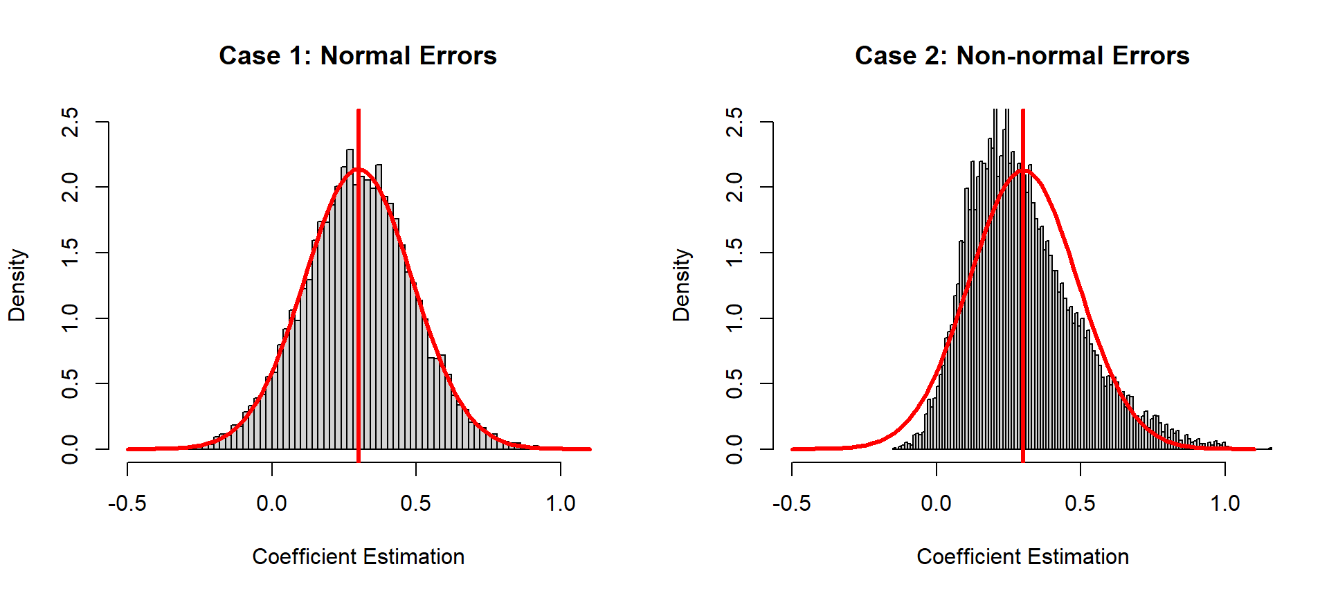
Let’s look at the distributions of the two results.

# The estimates are normally distributed in Case 1
hist(results1$est, breaks=100, freq=FALSE,
     xlim=c(-0.5, 1.1), ylim=c(0, 2.5),
     main='Case 1: Normal Errors', xlab='Coefficient Estimation')
curve(dnorm(x, mean=mean(results1$est), sd=sd(results1$est)),
      col='red', lwd=3, add=TRUE)
abline(v=0.3, col='red', lwd=3)

# The estimates are NOT normally distributed in Case 2
hist(results2$est, breaks=100, freq=FALSE,
     xlim=c(-0.5, 1.1), ylim=c(0, 2.5),
     main='Case 2: Non-normal Errors', xlab='Coefficient Estimation')
curve(dnorm(x, mean=mean(results2$est), sd=sd(results2$est)),
      col='red', lwd=3, add=TRUE)
abline(v=0.3, col='red', lwd=3)

Now we can see differences. The distribution of estimated coefficients follows a normal distribution in Case 1, but not in Case 2. That means that in Case 2 we cannot apply hypothesis testing, which is based on a normal distribution (or related distributions, such as a t-distribution). When errors are not normally distributed, estimations are not normally distributed, and we can no longer use p-values to decide if the coefficient is different from zero. In short, if the normality assumption of the errors is not met, we cannot draw a valid conclusion based on statistical inference in linear regression analysis.

And even then those procedures are actually pretty robust to violations of normality. In our second example above, our simulated sample size was 30 (kind of small) and our errors were drawn from a chi-square distribution with 1 degree of freedom. (You can't get any more non-normal than that!) And yet the sampling distribution histogram of the coefficient was not as far from normal as you might expect. Now if your sample is small (less than 30) and you detect extremely non-normal errors, you might consider alternatives to constructing standard errors and p-values, such as bootstrapping. But otherwise you can probably rest easy if your errors seem "normal enough."

Okay, I understand my variables don’t have to be normal. Why do we even bother checking histograms before analysis then?

Although your data don’t have to be normal, it’s still a good idea to check data distributions just to understand your data. Do they look reasonable? Your data might not be normal for a reason. Is it count data or reaction time data? In such cases, you may want to transform it or use other analysis methods (e.g., generalized linear models or nonparametric methods). The relationship between two variables may also be non-linear (which you might detect with a scatterplot). In that case transforming one or both variables may be necessary.

Summary

None of your observed variables have to be normal in linear regression analysis, which includes t-test and ANOVA. The errors after modeling, however, should be normal to draw a valid conclusion by hypothesis testing.

Note: There are other analysis methods that assume multivariate normality for observed variables (e.g., structural equation modeling).

Bommae Kim
Statistical Consulting Associate
University of Virginia Library
September 14, 2015