Understanding Somers' D

When it comes to summarizing the association between two numeric variables, we can use Pearson or Spearman correlation. When accompanied with a scatterplot, they allow us to quantify association on a scale from -1 to 1. But what if we have two ordered categorical variables with just a few levels? How can we summarize their association? One approach is to calculate Somers’ Delta, or Somers’ D for short.

To present Somers’ D, we’ll work with data from Agresti (2002). Below we create a table in R that cross-classifies income (in thousands of dollars) and job satisfaction for a sample of black males from the 1996 General Social Survey. The ordered levels of satisfaction are Very Dissatisfied (VD), Little Dissatisfied (LD), Moderately Satisfied (MS), and Very Satisfied (VS). Notice we could think of income as the independent variable and job satisfaction as the dependent variable. This is an important distinction to make when calculating Somers’ D.

# Table 2.8, Agresti (2002) p. 57
M <- as.table(rbind(c(1, 3, 10, 6), 
                    c(2, 3, 10, 7),
                    c(1, 6, 14, 12),
                    c(0, 1, 9, 11)))
dimnames(M) <- list(`income` = c("<15", "15-25", "25-40", ">40"),
                    `job satisfaction` = c("VD", "LD", "MS","VS"))
M

       job satisfaction
income  VD LD MS VS
  <15    1  3 10  6
  15-25  2  3 10  7
  25-40  1  6 14 12
  >40    0  1  9 11

There appears to be some association between income and satisfaction. For example, we see higher counts of Very Satisfied for higher income levels. We would like to quantify this association in some way. One way to do this is by looking at pairs of observations.

Consider a pair of subjects, one of whom earned income in the 15-25 range and answered Moderately Satisfied (MS), and another who earned income in the >40 range and answered Very Satisfied (VS). We say this pair of subjects is concordant. The subject with higher income also has higher satisfaction.

Now consider another pair of subjects, one of whom earned income in the 15-25 range and answered Moderately Satisfied (MS), and another who earned income in the >40 range but answered Little Dissatisfied (LD). We say this pair of subjects is discordant. The subject with higher income had lower satisfaction.

Finally we can have pairs of subjects that are neither concordant nor discordant, but tied on the independent variable. For example, we may have two subjects who both earned income in the 15-25 range, but one who answered Moderately Satisfied (MS) while the other answered Very Satisfied (VS). In this case, the two subjects are tied on income level.

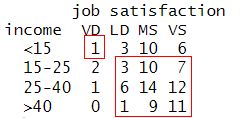
Let’s count up these different pairs for our data. First we’ll do the concordant pairs. The basic idea is to take the product between the concordant counts. Starting in the upper left corner of the cross-classified income table (<15 thousand, Very Dissatisfied), we show the first set of concordant pairs.

We can calculate the total number of pairs as follows:

M[1,1]*sum(M[2:4,2:4])

[1] 73

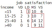
Moving left to right, the next set of concordant pairs are the following:

Again we can count the total number pairs as before using different indexing:

M[1,2]*sum(M[2:4,3:4])

[1] 189

We can follow this pattern and laboriously count the total number of concordant pairs, which comes out to 1331.

M[1,1]*sum(M[2:4,2:4]) +
  M[1,2]*sum(M[2:4,3:4]) +
  M[1,3]*sum(M[2:4,4:4]) +
  M[2,1]*sum(M[3:4,2:4]) +
  M[2,2]*sum(M[3:4,3:4]) +
  M[2,3]*sum(M[3:4,4:4]) +
  M[3,1]*sum(M[4:4,2:4]) +
  M[3,2]*sum(M[4:4,3:4]) +
  M[3,3]*sum(M[4:4,4:4])

[1] 1331

We could automate this process using nested for loops and indexing. Fortunately, the {DescTools} package provides the ConDisPairs() function to do this for us. If you don’t have this package, you can install it by running install.packages("DescTools"). Below we call ConDisPairs() on the table and save the result as “pair_counts”. The result is a list of four objects. The “C” element contains the concordant counts, which comes to 1331.

# install.packages("DescTools")
library(DescTools)
pair_counts <- ConDisPairs(M)
Concordant <- pair_counts$C
Concordant

[1] 1331

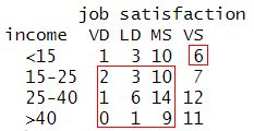
We count discordant pairs in a similar fashion. Below we highlight the first set of discordant pairs starting in the upper right corner of the table.

Moving right to left, we can continue to identify discordant pairs using the same pattern, but in the opposite direction, that we used to identify concordant pairs. Instead of demonstrating this, we’ll extract the discordant counts from our “pair_counts” object we created above, which is available in the “D” element. The total comes out to 849.

Discordant <- pair_counts$D
Discordant

[1] 849

Next we count the total number of pairs tied on the independent variable, income. First we sum the counts in each row, and then for each row total, find the total number of all possible pairs using the choose() function. ¹ We then total up all those counts.

Ties <- sum(apply(M, 1, function(x)choose(n = sum(x), k = 2)))
Ties

[1] 1159

And finally we count up all possible pairs in our data using choose().

Total <- choose(sum(M), 2)
Total

[1] 4560

Now let’s use these various counts of pairs to quantify association in our table. To do this we’ll create a ratio. In the numerator we’ll take the difference between concordant and discordant pairs. In the denominator we’ll take the difference between all possible pairs and those pairs tied on income, the independent variable.

(Concordant - Discordant)/ (Total - Ties)

[1] 0.141723

This is the Somers’ D statistic. This says, “of all the pairs in our data (minus those tied on income), the proportion of concordant pairs is about 0.14 higher than the proportion of discordant pairs.” The association in this case appears to be positive but weak. It’s important to note that the difference in the numerator can be negative, which would mean a surplus of discordant pairs and a negative Somers’ D statistic. This implies Somers’ D can range from -1 to 1. This also indicates that when there is no difference in the number of concordant and discordant pairs, the numerator will be 0 and imply no association between the variables.

We can formally summarize our work above using the following expression,

\[d = \frac{C - D}{{n \choose 2} - \sum_{i=1}^{k} {n_i \choose 2}} \]

where C = number of concordant pairs, D = number of discordant pairs, \({n \choose 2}\) is the number all pairs, and \(\sum_{i=1}^{k} {n_i \choose 2}\) is the total number of pairs tied on each of the k rows of the independent variable.

You’ll be happy to know the {DescTools} package provides the SomersDelta() function to carry out this calculation for us. The direction argument tells the function where the dependent variable is located. The default is “row”. We specify “column” since our dependent variable, job satisfaction, is located on the columns.

SomersDelta(M, direction = "column")

[1] 0.141723

The SomersDelta() function also includes a conf.level argument that allows us to calculate a confidence interval on Somers’ D.

SomersDelta(M, direction = "column", conf.level = 0.95)

      somers       lwr.ci       upr.ci 
 0.141723023 -0.008008647  0.291454693 

The data are consistent with a Somers’ D ranging from about 0 to 0.29. The association is not only weak but very uncertain.

The Somers’ D statistic is a modification of the Gamma statistic, which makes no distinction between independent and dependent variables. Using our counts of concordant and discordant pairs above, we can easily calculate the Gamma statistic. It’s simply the difference in concordant and discordant pairs divided by the total of concordant and discordant pairs.

(Concordant - Discordant)/(Concordant + Discordant)

[1] 0.2211009

Or use the {DescTools} GoodmanKruskalGamma() function:

GoodmanKruskalGamma(M)

[1] 0.2211009

Since the Gamma statistic does not account for ties, it tends to exaggerate the actual strength of association. However it may be more suitable if we can’t plausibly identify one of our variables as “depending” on the other.

Somers’ D is frequently used with binary logistic regression models to quantify the association between the observed and predicted outcomes. This may seem strange given that we just presented Somers’ D as a way to summarize association between two ordered categorical variables. But if we imagine predicted probabilities as an ordered category and the observed binary 0/1 response as an ordered category, the Somers’ D statistic becomes a nice way to quantify the ability of the model to correctly discriminate between pairs of observations. In this scenario, we imagine our binary 0/1 response as the independent variable and the predicted probability as the dependent variable. A good model would mean lots of concordant pairs of data, where subjects observed as a 1 have a higher probability than subjects observed as a 0. A Somers’ D of 1 would mean our model perfectly discriminates and a value of 0 would mean our model is no better than flipping a fair coin. Let’s work a toy example.

Below we manually generate data on four subjects. For each subject we present their observed binary response and their predicted probability based on some imaginary logistic regression model:

\[\{0, 0.2\},\{0, 0.2\},\{1, 0.2\},\{1, 0.8\} \]

The first and second subjects have an observed binary response of 0 and predicted probabilities of 0.2. The third subject has an observed binary response of 1 and a predicted probability of 0.2. The fourth subject has an observed binary response of 1 and a predicted probability of 0.8. We can eyeball these four subjects and see that we have two concordant pairs: the two instances of \(\{0,0.2\}\) versus \(\{1,0.8\}\). We can also see we have no discordant pairs. That is, we don’t have any instances of someone with an observed 0 having a higher predicted probability than someone with an observed 1. Therefore we have a surplus of concordant pairs and a positive Somers’ D. We can can calculate this by hand.

• Concordant pairs = 2
• Discordant pairs = 0
• Pairs tied on observed response = 2 (first two subjects both have 0, second two subjects both have 1, therefore two pairs tied on the observed response)
• All tied pairs: \({4 \choose 2} = 6\)

\[\frac{2 - 0}{6 - 2} = \frac{2}{4}- \frac{0}{4} = \frac{1}{2}\]

The proportion of concordant pairs is 0.5 higher than the proportion of discordant pairs.

We can also calculate Somer’s D for this toy example by entering the data as vectors, cross-classifying the vectors using the table() function, and calling SomersDelta() on the result.

obsv_y <- c(0, 0, 1, 1)
pred_y <- c(0.2, 0.2, 0.2, 0.8)
M2 <- table(obsv_y, pred_y)
SomersDelta(M2, direction = "column")

[1] 0.5

Notice we specified direction = "column" to indicate that the predicted probabilities are considered the dependent variable.

Let’s fit a non-trivial binomial logistic regression model to see Somers’ D in action with some realistic data. Below we use the birthwt data set from the {MASS} package to model the probability of low infant birth weight as a function of hypertension history in mother (ht), previous premature labor (ptl), and mother’s weight in pounds at last menstrual period (lwt).

library(MASS)
data("birthwt")
# convert ptl to indicator
birthwt$ptl <- ifelse(birthwt$ptl < 1, 0, 1)
m <- glm(low ~ ht + ptl + lwt, family = binomial, 
         data = birthwt)
summary(m)

Call:
glm(formula = low ~ ht + ptl + lwt, family = binomial, data = birthwt)

Coefficients:
             Estimate Std. Error z value Pr(>|z|)   
(Intercept)  1.017367   0.853337   1.192  0.23317   
ht           1.893971   0.721090   2.627  0.00863 **
ptl          1.406770   0.428501   3.283  0.00103 **
lwt         -0.017280   0.006787  -2.546  0.01090 * 
---
Signif. codes:  0 '***' 0.001 '**' 0.01 '*' 0.05 '.' 0.1 ' ' 1

(Dispersion parameter for binomial family taken to be 1)

    Null deviance: 234.67  on 188  degrees of freedom
Residual deviance: 210.12  on 185  degrees of freedom
AIC: 218.12

Number of Fisher Scoring iterations: 4

Judging from the summary output, it appears history of hypertension (ht) and previous instances of premature labor (ptl) are meaningfully associated with a higher probability of low infant birth weight. And we see the residual deviance is much lower than the null deviance, indicating this model is an improvement over simply using the proportion of low birth weight babies as our predicted probability. But how well might this model perform in a clinical setting? Ideally it would assign higher probability of low infant birth weight to a mother at risk than to a mother who is not. This is what Somers’ D can help us assess.

To calculate Somers’ D we need to first use our model to generate predicted probabilities. We can do that with the predict() function.

pred_low <- predict(m, type = "response")

Then we cross-classify predicted probabilities and the observed response and use SomersDelta() to carry out the calculation.

tab <- table(birthwt$low, pred_low)
SomersDelta(tab, direction = "column")

[1] 0.4378096

It appears we have a decent surplus of concordant pairs, about 0.44. This means given a pair of subjects, one with low = 0 and the other with low = 1, our model is usually predicting a higher probability for subjects with low = 1.

It’s worth noting that this Somers’ D statistic is almost certainly too optimistic. We calculated it using the same data we used to fit the model. To get a more realistic estimate of how the model might perform “in the wild”, we might consider using bootstrap model validation.

It turns out that Somers’ D has an interesting relationship with the AUC (Area Under the Curve) statistic:

\[\text{Somers' D} = 2(\text{AUC} - 0.5)\]

Whereas a Somers’ D of 0 indicates no ability to discriminate between pairs, the associated AUC value is 0.5. We see in the formula above that an AUC of 0.5 is equivalent to a Somers’ D of 0.

Let’s verify this relationship by calculating AUC for our model and then use the formula above to calculate Somers’ D. Below we use the auc() and roc() functions from the {pROC} package to calculate AUC.

# install.packages("pROC")
library(pROC)
AUC <- auc(roc(birthwt$low, pred_low))
2 * (AUC - 0.5) # Somers' D

[1] 0.4378096

The somers2() function from the {Hmisc} package calculates both statistics. The AUC is labeled “C” and Somers’ D is labeled “Dxy”.

# install.packages("Hmisc")
library(Hmisc)
somers2(pred_low, birthwt$low)

          C         Dxy           n     Missing 
  0.7189048   0.4378096 189.0000000   0.0000000 

For a gentle introduction to AUC as well as some helpful advice about using model performance metrics in general, we recommend the StatLab Article, ROC Curves and AUC for Models Used for Binary Classification.

Clay Ford
Statistical Research Consultant
University of Virginia Library
November 29, 2023

References

- Agresti A. (2002). Categorical data analysis. 2nd Ed. Wiley-Interscience.
- Harrell Jr, F. (2023). Hmisc: Harrell Miscellaneous. R package version 5.1-0, https://CRAN.R-project.org/package=Hmisc.
- R Core Team (2023). R: A Language and Environment for Statistical Computing. R Foundation for Statistical Computing, Vienna, Austria. https://www.R-project.org/.
- Robin X., Turck N., Hainard A., Tiberti N., Lisacek F., Sanchez J. and Müller M. (2011). pROC: an open-source package for R and S+ to analyze and compare ROC curves. BMC Bioinformatics, 12, p. 77. DOI: 10.1186/1471-2105-12-77 http://www.biomedcentral.com/1471-2105/12/77/
- Signorell A. (2023). DescTools: Tools for Descriptive Statistics. R package version 0.99.50, https://CRAN.R-project.org/package=DescTools.
- Somers R. H. (1962), A New Asymmetric Measure of Association for Ordinal Variables, American Sociological Review, 27, 799-811.
- Venables W. N. & Ripley B. D. (2002). Modern applied statistics with S. 4th Ed. Springer, New York. ISBN 0-387-95457-0.