Bootstrapping Residuals for Linear Models with Heteroskedastic Errors Invites Trouble

Bootstrapping—resampling data with replacement and recomputing quantities of interest—lets analysts approximate sampling distributions for complex estimators and frees them of the reliably unmet assumptions of traditional, parametric inferential statistics. It’s an elegant, intuitive approach in which an analyst exploits the (often) parallel resample-to-sample and sample-to-population relationships to understand uncertainty in an estimate.

In the context of regression, analysts frequently bootstrap to generate confidence intervals for coefficients and conditional means, as well as prediction intervals for future observations. The term “bootstrapping” is, in a way, slightly reductive, bundling into a single word an array of implementations and methods. Bootstrapping is not a fixed, identical scheme applied from data set to data set with minimal thought and maximal fervor. It’s a general approach, with resampling as its foundation. That resampling can take many forms. When working with a linear model, two standard forms are case resampling and residual resampling.

Case resampling is straightforward:

• Resample N cases with replacement from a data set containing N original cases
• Recompute a model or statistic using the bootstrapped data set; save the estimate(s) of interest
• Repeat the process B times

Residual resampling takes a different tack:

• Using a regression model fit to an original data set containing N cases, calculate predicted values for those N cases
• Resample N residuals with replacement from the original model
• Add the N residuals to the N predicted outcome values (thereby generating a “new” data set with updated outcome values)
• Recompute a model or statistic using the bootstrapped data set; save the estimate(s) of interest
• Repeat the process B times

The B bootstrap estimates approximate a sampling distribution for the quantity of interest. From that distribution, one can compute confidence intervals for the quantity (for example, a 95% percentile confidence interval comprises the .025 and .975 quantiles of the bootstrap estimates).¹

Both case and residual bootstrapping are useful when linear model errors are non-normal: Empirically estimating the distributions of regression coefficients via bootstrapping sidesteps the use of equations that only hold when errors are normal. Well-behaved, normal errors with constant variance gift Gaussianity to the coefficient distributions and render traditional, parametric equations for analytically estimating their properties valid (see Shalizi, 2019, pp. 380–381, and this StatLab article on robust standard errors), but the equations give biased results—like underestimated standard errors—when linear model errors are no longer given by \(\epsilon \sim N(0, \sigma^2)\).

When both kinds of boostrapping are applied to the same data set, residual resampling generally produces a slightly tighter sampling distribution, resulting in narrower confidence intervals (Davison & Hinkley, 1997, p. 264; Shalizi, 2024, p. 155). Why not, then, always opt for residual bootstrapping, or at least treat it as the default? Narrow bounds on confidence intervals are certainly attractive.

Residual bootstrapping for linear regression requires a pair of additional assumptions that case bootstrapping does not: (1) that model errors are identically distributed (homoskedastic), whatever their shape, and (2) that the relationship between the conditional mean of \(y\) and the predictors, \(x_1, x_2, ..., x_j\), is indeed linear. When generating a bootstrap sample via residual resampling, one begins by computing the predicted value for each original observation based on an initial (linear) model, \(\hat{y}_i, i = 1, 2, ..., n\). Residuals are then randomly plucked with replacement from the initial model, \(e^*_i, i = 1, 2, ... n\), and added to the predicted values to construct a bootstrapped data set. We act as though any residual can be validly paired up with any predicted value—as though the error distribution is independent of \(x_1, x_2, ..., x_j\) (and therefore independent of the conditional mean of \(y\)).

But the errors may well not be identically distributed. Perhaps, for example, \(y = x + \epsilon,~\epsilon \sim N(0, x)\). Acting as though residuals are all interchangeable—hot-swappable injections of uncertainty into \(\hat{y}_i\)—is no longer appropriate. Residual resampling ignores the inherent heteroskedasticity in the errors, and as a result, the bootstrapped data sets don’t adequately approximate samples from the population of interest. With case resampling, we avoid assumptions both about the shape of the error distribution and the constancy of it; residuals don’t make an appearance in the resampling process or in the computation of coefficients.²

I developed a simulation to investigate the relative performance of residual and case bootstrapping when model errors are not identically distributed. The outcome of interest was the coverage rate of 95% percentile confidence intervals generated by each bootstrapping method at several different “levels” of heteroskedasticity in the model errors, \(L \in \{0, 0.5, ..., 5.0\}\). At each level, I generated 1000 data sets containing 250 observations simulated via the linear equation \(y = x + \epsilon\), with \(x\) distributed as \(U(1, 5)\) and errors distributed as \(N(0, (x^L)^{2})\). I repeated this process 1000 more times for each \(L\), generating data sets with \(N = 250\) via the same linear equation but with errors now distributed as \(U(-1x^L, x^L)\). (I performed the simulation for normal and uniform errors to demonstrate that what matters is not normality itself, but rather the constancy of the error distribution across predictor values.) I bootstrapped each data set 2500 times with case resampling and 2500 times with residual resampling. I determined the 95% percentile bootstrap confidence interval given by each resampling method for each data set, checked if it included 1.0 (the true coefficient value), and saved the results. The plot shows the proportion of 95% confidence intervals that captured the parameter value for each resampling method, residual distribution, and level of residual heteroskedasticity The plot displays results from a total of 110,000,000 bootstrapped data sets.

library(doParallel)
library(doRNG)
library(ggplot2)

# Recruit several computer cores for parallelizing
registerDoParallel(cores = detectCores() - 1)
registerDoRNG(seed = 444)

cat('This simulation is parallelized over', detectCores() - 1, 'cores on my machine.\n')

This simulation is parallelized over 9 cores on my machine.

#######################################################################
# Warning: The simulation takes hours to run. If you want to test and #
# tweak the code without waiting for the full-scale simulation to     #
# complete, reduce the values of the k_boots and b objects below.     #
#######################################################################

# Establish simulation conditions and prepare object to iterate over in parallel foreach loop
lvl <- seq(from = 0, to = 5, by = 0.5)
k_boots <- 1000
b <- 2500
n <- 250
res_dist_normal <- c(TRUE, FALSE)
iters <- expand.grid(1:k_boots, lvl, res_dist_normal)
colnames(iters) <- c('k', 'lvl', 'res_dist_normal')

# Simulation results saved to matrix `out`
# foreach/%dopar% parallelizes the work over the recruited cores
out <- foreach (j = 1:nrow(iters), .combine = rbind, .inorder = FALSE) %dopar% {
  x <- runif(n, 1, 5)
  y <- 1*x +
    if (iters[j, 'res_dist_normal'] == TRUE) {
      rnorm(n, 0, x^iters[j, 'lvl'])
    } else {
      runif(n, -(x^iters[j, 'lvl']), x^iters[j, 'lvl'])
    }
  m <- lm(y ~ x)
  d <- data.frame(x, y)

  out_case <- foreach (i = 1:b, .combine = c, .inorder = FALSE) %do% {
    d_tmp <- d[sample(nrow(d), nrow(d), T), ]
    m_tmp <- lm(y ~ x, d_tmp)
    coef(m_tmp)[2]
  }

  out_res <- foreach (i = 1:b, .combine = c, .inorder = FALSE) %do% {
    d_tmp <- d
    d_tmp$y <- predict(m, d) + sample(resid(m), length(resid(m)), T)
    m_tmp <- lm(y ~ x, d_tmp)
    coef(m_tmp)[2]
  }

  # as.vector() strips elements names returned by quantile()
  as.vector(c(iters[j, 'lvl'], iters[j, 'res_dist_normal'],
              quantile(out_case, .025) < 1 && quantile(out_case, .975) > 1,
              quantile(out_res, .025) < 1 && quantile(out_res, .975) > 1))
}

# Reshape and aggregate results for plotting
out <- data.frame(out)
colnames(out) <- c('lvl', 'res_dist', 'case_boot_ci_captures', 'res_boot_ci_captures')
out$res_dist <-  ifelse(out$res_dist == TRUE, 'normal', 'uniform')
out_long <- tidyr::pivot_longer(out, cols = -c(lvl, res_dist), names_to = 'boot_method', values_to = 'captures')
to_plot <- aggregate(list(coverage_rate = out_long$captures),
                     by = list(boot_method = out_long$boot_method,
                               lvl = out_long$lvl,
                               res_dist = out_long$res_dist),
                     function(x) sum(x) / length(x))

# Define plotmath strings to be added to the facets of the plot
labs <- data.frame(res_dist = c('normal', 'uniform'),
                   lab_eq = c('y == x + epsilon', 'y == x + epsilon'),
                   lab_x = c('x %~% U(1, 5)', 'x %~% U(1, 5)'),
                   lab_res = c('epsilon %~% N(0, (x^L)^2)', 'epsilon %~% U(-1*x^L, x^L)'))

ggplot(to_plot, aes(lvl, coverage_rate, color = boot_method)) +
  geom_hline(yintercept = .95, alpha = .5) + geom_point() + geom_line() +
  facet_wrap(~res_dist, labeller = as_labeller(function(x) {
    paste0('Errors: ', gsub('(^\\w{1})', '\\U\\1', x, perl = T)) } )) +
  scale_color_manual(values = c('cornflowerblue', 'salmon'),
                     labels = c('Case bootstrap', 'Residual bootstrap')) +
  labs(title = paste0('95% Percentile Bootstrap Confidence Interval Coverage Rates by ',
                      'Bootstrap Method, Level of\nError Heteroskedasticity, ',
                      'and Shape of Error Distribution'),
       x = '\nLevel of error heteroskedasticity (L)',
       y = '95% CI coverage rate',
       color = 'Bootstrap method',
       caption = '2500 bootstraps performed on each of 1000 N=250 data sets at each value of L') +
  scale_x_continuous(breaks = lvl, labels = paste0('L=', lvl)) +
  scale_y_continuous(breaks = seq(0, 1, .2), labels = as.character(seq(0, 1, .2)), limits = c(0, 1)) +
  theme_bw() + theme(legend.position = 'bottom', panel.grid.minor = element_blank()) +
  geom_text(data = labs, aes(median(lvl), .40, label = lab_eq), color = 'black', parse = TRUE) +
  geom_text(data = labs, aes(median(lvl), .30, label = lab_x), color = 'black', parse = TRUE) +
  geom_text(data = labs, aes(median(lvl), .20, label = lab_res), color = 'black', parse = TRUE)

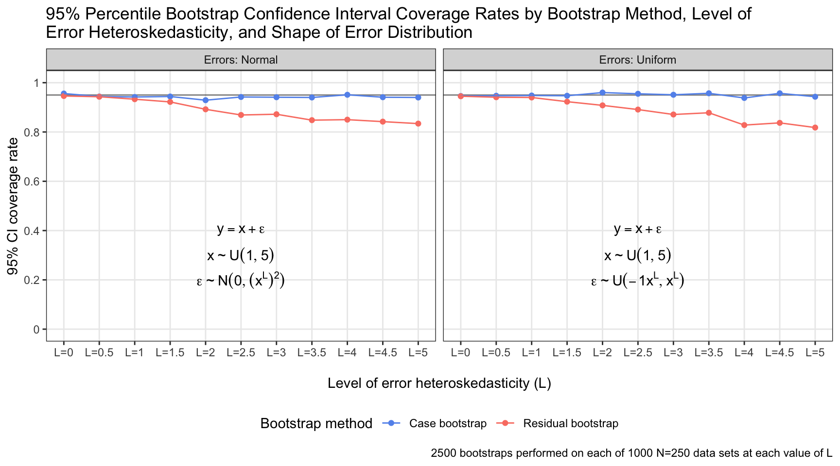
The coverage rate of 95% confidence intervals generated by residual bootstrapping decayed distinctly as the the error distribution became increasingly heteroskedastic (i.e., as \(L\) increased). Conversely, the coverage rate was quite stable for confidence intervals generated by case bootstrapping, regardless of \(L\). The specific shape of the error distribution was unimportant: Both residual and case bootstrapping retained close-to-nominal coverage rates (~95%) for normal and uniform identically distributed errors; it was the constancy of the distribution across the value of \(x\) that made the difference.

The simulation conditions underlying some of the results above are surely unrealistic: At the extreme, I assessed a case in which errors were distributed as \(\epsilon \sim N(0, (1^5)^{2} = 1)\) when \(x\) was at its minimum (1) and \(\epsilon \sim N(0, (5^5)^{2} = 9765625)\) when \(x\) was at its maximum (5). Where one would find such a data set in the wild, I do not know. But even for lower levels of heteroskedasticity, the coverage rates of confidence intervals derived from residual bootstrapping were disappointing. With \(L = 1.5\) and normally distributed errors, the error standard deviation was \(1^{1.5} = 1\) when \(x\) was at its minimum and \(5^{1.5} = 11.18\) when \(x\) was at its maximum. This is a (relatively) more plausible circumstance, and residual bootstrapping exhibited a coverage rate of 92%. And regardless: The nominal coverage rate should be the in-practice coverage rate; deviations are undesirable—and in this case, avoidable.

I prefer to err on the side of inferential caution, being more worried about making too many constrictive modeling assumptions than about being too analytically conservative. Bootstrapping cases is more in accordance with that philosophy than bootstrapping residuals,³ and my code, more often than not, reflects that.

References

• Davison, A. C., & Hinkey, D. V. (1997). Bootstrap methods and their applications. Cambridge University Press.
• Fox, J. (2015). Applied regression analysis and generalized linear models (3rd ed.). Sage.
• Shalizi, C. R. (2024, January 22). Advanced data analysis from an elementary point of view. https://www.stat.cmu.edu/~cshalizi/ADAfaEPoV/ADAfaEPoV.pdf
• Shalizi, C. R. (2019, November 2). The truth about linear regression. https://www.stat.cmu.edu/~cshalizi/TALR/TALR.pdf

Jacob Goldstein-Greenwood
Research Data Scientist
University of Virginia Library
February 02, 2024