Stata Tip: Name Your Graphs

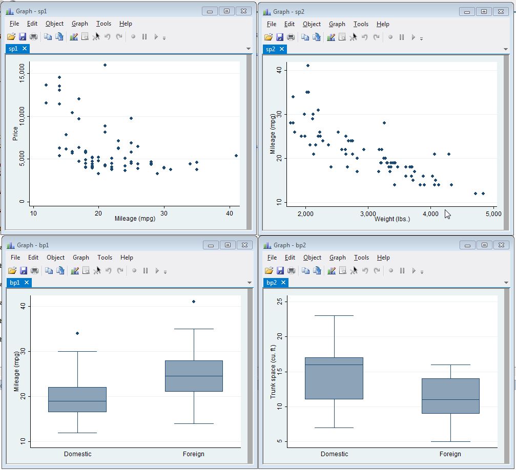
An important component of data analysis is graphing. Stata provides excellent graphics facility for quickly exploring and visualizing your data. For example, let's load the auto data set that comes with Stata (1978 Automobile Data) and make two scatterplots and then two boxplots:

sysuse auto
twoway scatter price mpg
twoway scatter mpg weight
graph box mpg, over(foreign)
graph box trunk, over(foreign)

If you open Stata and run those commands, you'll notice each new graph overwrites the previous graph. In fact if you submit all five lines from a do file (ie, highlight all lines and click Ctrl + D), you'll only see the last box plot. That's annoying if you want to see multiple graphs at the same time. This is where naming your graphs comes in handy.

To name your graph, use the name option. Close the boxplot window (if you ran the commands above) and reissue the first graphing command above with the name option:

twoway scatter price mpg, name(sp1)

Now the graph is saved in memory and accessible by the name sp1. (There's nothing special about the name sp1. We just made it up. We could have named it price_vs_mpg or blah. Name your graph whatever you want. Just make sure there are no spaces in the name.) If you close the graph, you can access it again using the syntax graph display sp1. Now that's not a terribly big deal since you could also just resubmit the original syntax to see the graph again. But it is a big deal when you have multiple graphs that you would like to view at the same time.

Leave the first scatterplot window open and reissue the second scatterplot syntax with a name option:

twoway scatter mpg weight, name(sp2)

Now both graphs are displayed. The second graph didn't overwrite the first! (In Windows you may have to move the 2nd graph to see the 1st one.) As long as we keep naming subsequent graphs, they will appear in their own window. Let's name our box plots:

graph box mpg, over(foreign) name(bp1)
graph box trunk, over(foreign) name(bp2)

If you haven't closed your previous graphs, you should now have four Stata Graph windows open which you can easily arrange and compare side-by-side.

"But I hate having all those Graph windows open!" No worries. Stata offers the autotabgraphs option so all graphs appear in one window with multiple tabs. Before we demonstrate, we'll close the four Graph windows as follows:

graph close

That's much easier than manually closing each Graph window one at a time. Now we turn on the autotabgraphs option:

set autotabgraphs on

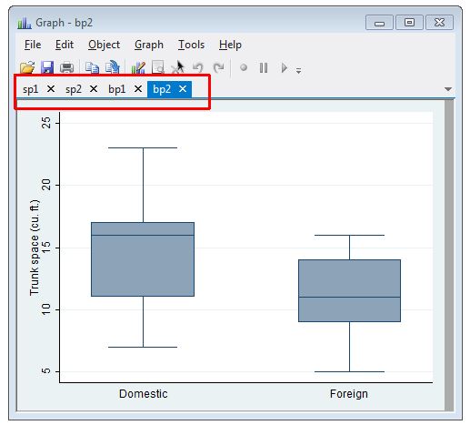
Now when we issue new graph commands with a name, the graphs appear in one window with tabs identifying the graph. What happens if we try to reissue one of our previous graph commands?

twoway scatter mpg price, name(sp1)

graph sp1 already exists

We get an error. You can't overwrite a named graph in memory. To see the graph, you have two options. (1) You can drop the sp1 graph from memory using drop graph sp1 and then reissue the original graphing syntax, or (2) you can issue the command graph display sp1 to view the saved graph.

Using the second option, we can quickly produce all four graphs in one window:

graph display sp1
graph display sp2
graph display bp1
graph display bp2

In the single window we can't compare graphs side-by-side, but we can easily switch between the graphs using Ctrl + Tab. Again, this is all thanks to naming our graphs. Having autotabgraphs turned on only produces multiple graphs in one window if you name your graphs! Otherwise each new graph overwrites the previous one.

Two other graph commands that are good to know:

• graph dir lists all graphs in memory.
• graph drop _all removes all graphs from memory.

References

StataCorp. 2015. Stata 13 Base Reference Manual. College Station, TX: Stata Press.

Clay Ford
Statistical Research Consultant
University of Virginia Library
August 7, 2015