Getting Started with the purrr Package in R

If you're wondering what exactly the purrr package does, then this blog post is for you.

Before we get started, we should mention the Iteration chapter in R for Data Science by Garrett Grolemund and Hadley Wickham. We think this is the most thorough and extensive introduction to the purrr package currently available (at least at the time of this writing.) Wickham is one of the authors of the purrr package, and he spends a good deal of the chapter clearly explaining how it works. Good stuff; recommended reading.

The purpose of this article is to provide a short introduction to purrr, focusing on just a handful of functions. We use some real world data and replicate what purrr does in base R so we have a better understanding of what's going on.

We visited Yahoo Finance on 13 April 2017 and downloaded about three weeks of historical data for three companies: Boeing, Johnson & Johnson, and IBM. The following R code will download and unzip the data in your current working directory if you wish to follow along.

URL <- "http://static.lib.virginia.edu/statlab/materials/data/stocks.zip"
download.file(url = URL, destfile = basename(URL))
unzip(basename(URL))

We have three .csv files. In the spirit of being efficient, we would like to import these files into R using as little code as possible (as opposed to calling read.csv() three different times.)

Using base R functions, we could put all the file names into a vector and then apply the read.csv() function to each file. This results in a list of three data frames. When done, we could name each list element using the names() function and our vector of file names.

# get all files ending in csv
files <- list.files(pattern = "csv$") 
# read in data
dat <- lapply(files, read.csv)
names(dat) <- gsub("\\.csv", "", files) # remove file extension

Here is how we do the same using the map() function from the purrr package.

install.packages("purrr") # if package not already installed
library(purrr)
dat2 <- map(files, read.csv)
names(dat2) <- gsub("\\.csv", "", files)

So we see that map() is like lapply(). It takes a vector as input and applies a function to each element of the vector. map() is one of the star functions in the purrr package.

Let's say we want to find the mean opening price for each stock. Here is a base R way using lapply() and an anonymous function:

lapply(dat, function(x)mean(x$Open))

$BA
[1] 177.8287

$IBM
[1] 174.3617

$JNJ
[1] 125.8409

We can do the same with map().

map(dat, function(x)mean(x$Open))

$BA
[1] 177.8287

$IBM
[1] 174.3617

$JNJ
[1] 125.8409

But map() allows us to bypass the function() function. Using a tilda (~) in place of function() and a dot (.) in place of x, we can do this:

map(dat, ~mean(.$Open))

Furthermore, purrr provides several versions of map() that allow you to specify the structure of your output. For example, if we want a vector instead of a list, we can use the map_dbl() function. The "_dbl" indicates that it returns a vector of type double (i.e., numbers with decimals).

map_dbl(dat, ~mean(.$Open))

      BA      IBM      JNJ 
177.8287 174.3617 125.8409 

Now let's say that we want to extract each stock's opening price data. In other words, we want to go into each data frame in our list and pull out the Open column. We can do that with lapply() as follows:

lapply(dat, function(x)x$Open)

$BA
 [1] 178.25 177.50 179.00 178.39 177.56 179.00 176.88 177.08 178.02 177.25 177.40 176.29 174.37 176.85 177.34 175.96 179.99
[18] 180.10 178.31 179.82 179.00 178.54 177.16

$IBM
 [1] 171.04 170.65 172.53 172.08 173.47 174.70 173.52 173.82 173.98 173.86 174.30 173.94 172.69 175.12 174.43 174.04 176.01
[18] 175.65 176.29 178.46 175.71 176.18 177.85

$JNJ
 [1] 124.54 124.26 124.87 125.12 124.85 124.72 124.51 124.73 124.11 124.74 125.05 125.62 125.16 125.86 126.10 127.05 128.38
[18] 128.04 128.45 128.44 127.05 126.86 125.83

Using map() is a little easier. We just provide the name of the column we want to extract.

map(dat, "Open")

$BA
 [1] 178.25 177.50 179.00 178.39 177.56 179.00 176.88 177.08 178.02 177.25 177.40 176.29 174.37 176.85 177.34 175.96 179.99
[18] 180.10 178.31 179.82 179.00 178.54 177.16

$IBM
 [1] 171.04 170.65 172.53 172.08 173.47 174.70 173.52 173.82 173.98 173.86 174.30 173.94 172.69 175.12 174.43 174.04 176.01
[18] 175.65 176.29 178.46 175.71 176.18 177.85

$JNJ
 [1] 124.54 124.26 124.87 125.12 124.85 124.72 124.51 124.73 124.11 124.74 125.05 125.62 125.16 125.86 126.10 127.05 128.38
[18] 128.04 128.45 128.44 127.05 126.86 125.83

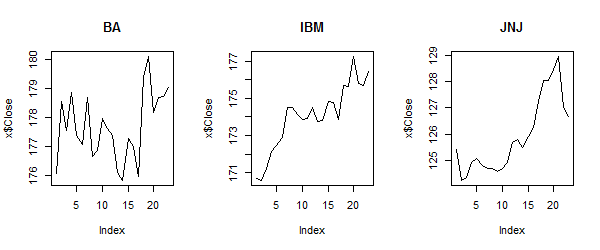
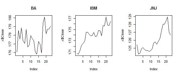
We often want to plot financial data. In this case we may want to plot the closing price for each stock and look for trends. We can do this with the base R function mapply(). First we create a vector of stock names for plot labeling. Next we set up one row of three plotting regions. Then we use mapply() to create the plot. The "m" in mapply means "multiple arguments." In this case we have two arguments: the closing price and the stock name. Notice that mapply() requires the function come first and then the arguments.

stocks <- sub("\\.csv","", files)
par(mfrow=c(1,3))
mapply(function(x,y)plot(x$Close, type = "l", main = y), x = dat, y = stocks)

The purrr equivalent is map2(). Again we can substitute a tilda (~) for function(), but now we need to use .x and .y to identify the arguments. However, the ordering is the same as map(): Data come first, and the function follows.

map2(dat, stocks, ~plot(.x$Close, type="l", main = .y))

Each time we run mapply() or map2() above, the following is printed to the console:

$BA
NULL

$IBM
NULL

$JNJ
NULL

This is because both functions return a value. Since plot() returns no value, NULL is printed. The purrr package provides walk() for dealing with functions like plot(). Here is the same task with walk2() instead of map2(). It produces the plots and prints nothing to the console.

walk2(dat, stocks, ~plot(.x$Close, type="l", main = .y))

At some point we may want to collapse our list of three data frames into a single data frame. This means we'll want to add a column to indicate which record belongs to which stock. Using base R this is a two step process. We use the do.call() function with the rbind() function on the elements of our list. Then we add a column called Stock by taking advantage of the fact that the row names of our data frame contain the name of the original list element, in this case the stock name.

datDF <- do.call(rbind, dat)
# add stock names to data frame
datDF$Stock <- gsub("\\.[0-9]*", "", rownames(datDF)) # remove period and numbers
head(datDF)

           Date   Open   High    Low  Close  Volume Adj.Close Stock
BA.1 2017-04-12 178.25 178.25 175.94 176.05 2920000    176.05    BA
BA.2 2017-04-11 177.50 178.60 176.96 178.57 2259700    178.57    BA
BA.3 2017-04-10 179.00 179.97 177.48 177.56 2259500    177.56    BA
BA.4 2017-04-07 178.39 179.09 177.26 178.85 2704700    178.85    BA
BA.5 2017-04-06 177.56 178.22 177.12 177.37 2343600    177.37    BA
BA.6 2017-04-05 179.00 180.18 176.89 177.08 2387100    177.08    BA

Using purrr, we can accomplish this using the list_rbind() function with the argument names_to = "stock". The names_to argument takes the names of the list elements and copies them into a column with the name we provide, in this case stock.

dat2DF <- list_rbind(dat2, names_to = "stock")
head(dat2DF)

  stock       Date   Open   High    Low  Close  Volume Adj.Close
1    BA 2017-04-12 178.25 178.25 175.94 176.05 2920000    176.05
2    BA 2017-04-11 177.50 178.60 176.96 178.57 2259700    178.57
3    BA 2017-04-10 179.00 179.97 177.48 177.56 2259500    177.56
4    BA 2017-04-07 178.39 179.09 177.26 178.85 2704700    178.85
5    BA 2017-04-06 177.56 178.22 177.12 177.37 2343600    177.37
6    BA 2017-04-05 179.00 180.18 176.89 177.08 2387100    177.08

We can also do this using the dplyr function bind_rows(). Setting the .id argument to "stock" tells the function to create a column called stock using the names of the list elements.

dat2DF <- dplyr::bind_rows(dat2, .id = "stock")

Finally, let's return to the dat2 list and consider how to reformat the Date column as a date variable instead of a character variable. The easiest way to deal with this would have been to use the read_csv() function from the readr package instead of read.csv(). But in the interest of demonstrating some more purrr functionality, let's pretend we can't do that. Further, let's pretend we don't know which columns are character, but we would like to convert them to date if they are character. This time we give a purrr solution first.

To do this, we nest one function in another. The first one is modify_if(). This allows us to define a condition to dictate whether or not we modify a list element. In this case the condition is determined by is.character(). If is.character() returns TRUE, then we apply the ymd() function from the lubridate package. Notice we're applying modify_if() to each element of the data frames contained in dat2. But that's OK, because data frames are actually lists. So dat2 is a 3-item list, and each item is itself a list. Hence the reason we have nested functions. Below we map the modify_if() function to each list element, which is then mapped to each data frame column (or list element).

dat2 <- map(dat2, ~modify_if(., is.character, lubridate::ymd))

Doing this in base R is possible but far more difficult. We nest one lapply() function inside another, but since lapply() returns a list, we need to wrap the first lapply() with as.data.frame(). And within the first lapply() we have to use the assignment operator as a function, which works but looks cryptic!

dat <- lapply(dat, 
              function(x)as.data.frame(
                lapply(x,
                       function(y)
                         if(is.character(y)) 
                           `<-`(y, lubridate::ymd(y)) 
                       else y)))

This article provides just a taste of purrr. We hope it gets you started learning more about the package. Be sure to read the documentation as well. Each help page contains illustrative examples. Note that purrr is a very young package. At the time of this writing it is at version 0.2.2. There are sure to be improvements and changes in the coming months and years. This article has been updated for purrr version 1.0.1.

Clay Ford
Statistical Research Consultant
University of Virginia Library
April 14, 2017
Updated April 26, 2023

References

- R Core Team (2025). R: A Language and Environment for Statistical Computing. R Foundation for Statistical Computing, Vienna, Austria. https://www.R-project.org/.
- Wickham H, Henry L (2025). purrr: Functional Programming Tools. doi:10.32614/CRAN.package.purrr https://doi.org/10.32614/CRAN.package.purrr, R package version 1.2.0, https://CRAN.R-project.org/package=purrr.