If you have ever performed binary logistic regression in R using the glm() function, you may have noticed a summary of “Deviance Residuals” at the top of the summary output. In this article, we talk about how these residuals are calculated and what we can use them for. We also talk about other types of residuals available for binary logistic regression.
(June 2023 update: as of R version 4.3.0, the summary output of glm() objects no longer provides a summary of “Deviance Residuals”. However, deviance residuals can still be calculated and used for diagnostic purposes.)
To begin, let’s fit an example binary logistic regression model using the ICU (intensive care unit) data set that’s included with the vcdExtra package. Below we model the probability of dying once admitted to an adult ICU as a function of subject’s age and whether or not they were unconscious upon admission. We also reset the row numbering of the ICU data frame to make it easier to extract rows of interest later in this article.
library(vcdExtra)
data(ICU)
# reset the row numbering
rownames(ICU) <- NULL
m <- glm(died ~ age + uncons, data = ICU, family = binomial)
summary(m)
  Call:
  glm(formula = died ~ age + uncons, family = binomial, data = ICU)

  Deviance Residuals:
      Min       1Q   Median       3Q      Max
  -2.3128  -0.6231  -0.5140  -0.3226   2.4421

  Coefficients:
              Estimate Std. Error z value Pr(>|z|)
  (Intercept) -3.45771    0.80964  -4.271 1.95e-05 ***
  age          0.02778    0.01215   2.287   0.0222 *
  unconsYes    3.58783    0.79350   4.522 6.14e-06 ***
  ---
  Signif. codes:  0 '***' 0.001 '**' 0.01 '*' 0.05 '.' 0.1 ' ' 1

  (Dispersion parameter for binomial family taken to be 1)

      Null deviance: 200.16  on 199  degrees of freedom
  Residual deviance: 159.48  on 197  degrees of freedom
  AIC: 165.48

  Number of Fisher Scoring iterations: 5
At the top of the output, we see a section titled “Deviance Residuals,” which displays a five-number summary of the residuals. We can reproduce this summary by extracting the residuals and using the quantile() function.
quantile(residuals(m))
          0%        25%        50%        75%       100%
  -2.3127570 -0.6231176 -0.5140270 -0.3225848  2.4420598
In general, the reason we might be interested in this summary is to see how well our model is fitting the data. Residuals are the differences between what we observe and what our model predicts. It would be nice if our residuals were evenly distributed. We would like for the first quantile and third quantile values and minimum and maximum values to be about the same in absolute value, and for the median to be close to 0. In addition, we would like to see the minimum and maximum values be less than about 3 in absolute value. This is because deviance residuals can be roughly approximated with a standard normal distribution when the model holds (Agresti, 2002). Residuals greater than the absolute value of 3 are in the tails of a standard normal distribution and usually indicate strain in the model.
But recall that our response variable, died, takes two values, 0 and 1, and that our model is predicting a probability that ranges between 0 and 1. So how are we getting residuals such as -2.31 or 2.44?
It turns out there are a several residuals we can calculate from a binary logistic regression model. The most basic is the raw residual, which we’ll call \(e_i\). This is simply the difference between what we observe (\(y_i\)) and the predicted probability (\(\hat{p_i}\)). It ranges between -1 and 1.
$$e_i = y_i - \hat{p_i}$$
We can calculate these by hand. Notice we need to first convert our response to a 0 and 1. (It is stored as a factor in the ICU data frame.) When finished, we show the observed value (y), predicted probability from model (p_hat), and raw residual (e) for the first few observations.
p_hat <- predict(m, type = "response")
y <- ifelse(ICU$died == "Yes", 1, 0)
e <- y - p_hat
cbind(y, p_hat, e) |>
  head()
    y      p_hat           e
  1 0 0.06253121 -0.06253121
  2 0 0.13962618 -0.13962618
  3 0 0.21110650 -0.21110650
  4 0 0.12375704 -0.12375704
  5 0 0.26106920 -0.26106920
  6 0 0.17645557 -0.17645557
We can also get raw residuals using residuals() with type = "response".
# raw residuals
e <- residuals(m, type = "response")
Another type of residual is the Pearson residual. It is the raw residual divided by the estimated standard deviation of a binomial distribution with number of trials equal to 1 and p equal to \(\hat{p}\). The Pearson residual is basically a rescaled version of the raw residual. We’ll call it \(r_i\).
$$r_i = \frac{e_i}{\sqrt{\hat{p_i}(1 - \hat{p_i})}}$$
We can also calculate this by hand or use residuals() with type = "pearson".
r <- e / sqrt(p_hat * (1 - p_hat))
# or
r <- residuals(m, type = "pearson")
cbind(y, p_hat, r) |>
  head()
    y      p_hat          r
  1 0 0.06253121 -0.2582677
  2 0 0.13962618 -0.4028467
  3 0 0.21110650 -0.5172990
  4 0 0.12375704 -0.3758138
  5 0 0.26106920 -0.5943961
  6 0 0.17645557 -0.4628861
Yet another residual is the standardized Pearson residual. This is the Pearson residual adjusted for the leverage of predictors using what are called "hat values." Hat values measure the distance of individual predictors from the mean of the predictors. High hat values indicate a subject or row could have outlying predictor values. This in turn could mean that a subject or row has substantial leverage in determining the predicted response. This adjustment then increases the absolute value of certain residuals based on the leverage of the associated predictors. We’ll call this residual \(rs_i\).
$$rs_i = \frac{r_i}{\sqrt{1 - \hat{h_i}}}$$
We can calculate these by hand using the hatvalues() function, or by using the rstandard() function with type = "pearson".
rs <- r / sqrt(1 - hatvalues(m))
# or
rs <- rstandard(m, type = "pearson")
cbind(y, p_hat, rs) |>
  head()
    y      p_hat         rs
  1 0 0.06253121 -0.2601841
  2 0 0.13962618 -0.4040353
  3 0 0.21110650 -0.5202722
  4 0 0.12375704 -0.3770517
  5 0 0.26106920 -0.6014345
  6 0 0.17645557 -0.4645071
An interesting property of standardized Pearson residuals is that they have an approximate standard normal distribution if the model fits (Agresti, 2002). This can be useful for assessing model fit as we demonstrate later in the article.
Finally we come to deviance residuals, which we’ll call \(d_i\). These are based on a weird-looking formula derived from the likelihood ratio test for comparing logistic regression models, where we compare our current model to a saturated model. A saturated model is a model with as many coefficients as there are observations. The formula for calculating this test statistic for a single observation produces the deviance residual. Notice the sign of \(d_i\) is the same as that of \(e_i\).
$$d_i = \text{sign}(e_i) [-2(y_i \text{log}\hat{p_i} + (1 - y_i)\text{log}(1 - \hat{p_i}))]^{1/2}$$ We can calculate this by hand or just use the residuals() function. We use the sign() function to get the sign of \(e_i\).
d <- sign(e)*sqrt(-2*(y*log(p_hat) + (1 - y)*log(1 - p_hat)))
# or
d <- residuals(m)
cbind(y, p_hat, d) |>
  head()
    y      p_hat          d
  1 0 0.06253121 -0.3593656
  2 0 0.13962618 -0.5484311
  3 0 0.21110650 -0.6886566
  4 0 0.12375704 -0.5140270
  5 0 0.26106920 -0.7778830
  6 0 0.17645557 -0.6231176
Again, these are the deviance residuals we see summarized in the model summary output.1
If we square the deviance residuals and add them all up, we get the residual deviance statistic we see printed at the bottom of the summary output:
sum(d^2)
[1] 159.4783
We can also extract this from the model object with the deviance() function.
deviance(m)
[1] 159.4783
This test statistic can help us assess if our model is different from the saturated model. The null of the test is no difference between the models. The LRstats() function from the vcdExtra package runs this test for us. We fail to reject the null hypothesis in this case.
vcdExtra::LRstats(m)
  Likelihood summary table:
       AIC    BIC LR Chisq  Df Pr(>Chisq)
  m 165.48 175.37   159.48 197     0.9768
Deviance residuals measure how much probabilities estimated from our model differ from the observed proportions of successes. Bigger values indicate a bigger difference. Smaller values mean a smaller difference.
The smallest deviance residual is in row 23. The observed response is 0 (did not die), and the model predicts a small probability of dying. Hence we get a small deviance residual (i.e., close to 0).
i <- which.min(abs(residuals(m))) # 23
ICU$died[i]
  [1] No
  Levels: No Yes
p_hat[i]
          23
  0.04683521
residuals(m)[i]
          23
  -0.3097337
The largest deviance residual is in row 165. The observed response is a 1 (did die), but the model predicts a small probability of dying. Thus we have a large deviance residual.
i <- which.max(abs(residuals(m))) # 165
ICU$died[i]
  [1] Yes
  Levels: No Yes
p_hat[i]
         165
  0.05070007
residuals(m)[i]
      165
  2.44206
We mentioned the formula for deviance residuals is a bit weird. It uses log transformations and addition. Why is that? To better understand this, we need to talk about maximum likelihood. Consider the following toy example of flipping coins.
Let’s say we have a coin that lands heads 40% of the time (p = 0.4) and flip it 5 times (1 = heads, 0 = tails). We observe 1, 0, 1, 1, 0. The joint probability of getting this result is calculated as follows2:
p <- 0.4
p * (1 - p) * p * p * (1 - p)
[1] 0.0230
Or written more compactly using exponents:
(p^3)*(1-p)^2
[1] 0.02304
What if we didn’t know p? Our formula would look as follows:
$$\text{joint probability} = p^3 (1 - p)^2$$
One approach to finding p would be to try different values and select the one that maximizes the joint probability. In other words, what value of p would make the data we observed most likely? Let’s try 0.1 and 0.5.
p <- c(0.1, 0.5)
(p^3)*(1-p)^2
[1] 0.00081 0.03125
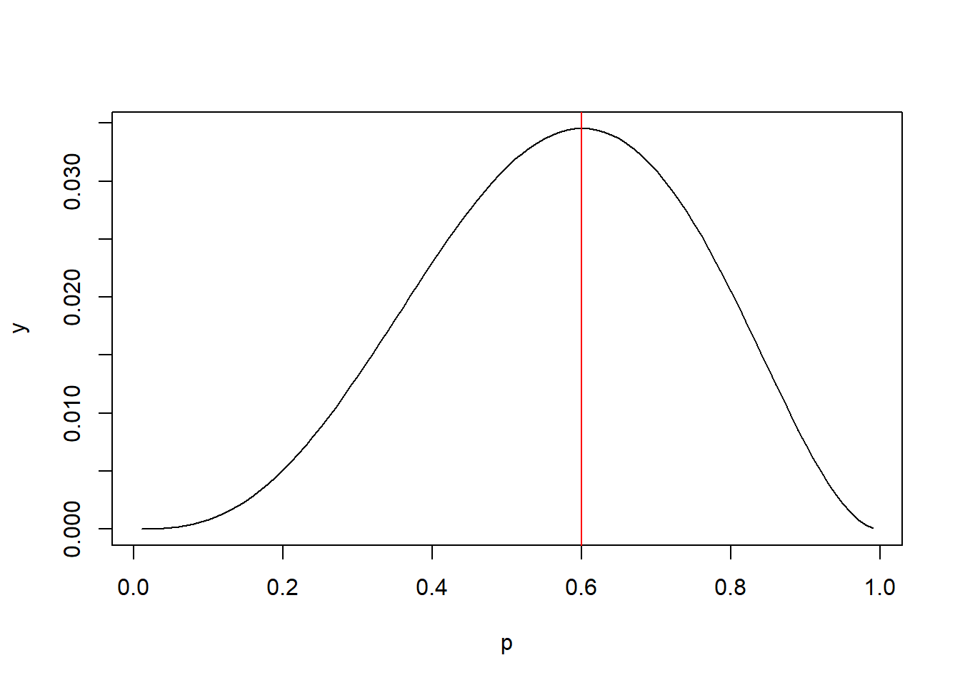
It looks like 0.5 is more likely than 0.1 because the joint probability is higher. Fortunately we don’t need to use trial and error. It can be shown that the value that maximizes the joint probability is simply the number of 1s divided by the number of trials: 3/5 or 0.6. So the most likely value of p for the binomial data we observed is 0.6. Sometimes this concept is presented visually by plotting the joint probabilities for various values of p versus p. Below we see the peak of the curve is at p = 0.6
p <- seq(0.01, 0.99, 0.01)
y <- (p^3)*(1-p)^2
plot(p, y, type = "l")
abline(v = 0.6, col = "red")

The value of the joint probability on the y-axis doesn’t really matter. We just want to know what p on the x-axis corresponds with the maximum value.
In the general case, we refer to joint probability as likelihood (\(L\)), with number of successes (\(s\)) and total number of trials (\(n\)).
$$L = p^s(1 - p)^{n-s}$$
If we log transform both sides of this equation we get log likelihood.
$$\log L = s\log(p) + (n - s)\log(1 - p)$$
We can also write this in terms of individual observations where \(y_i\) takes a value of 0 or 1. Notice this is similar to the formula we presented earlier for deviance residuals with \(n = 1\) and s equal to \(y_i\).
$$\log L = \sum_{i = 1}^{n} y_i\log(p) + (1 - y_i)\log(1 - p)$$
This is easier to compute since we’re adding instead of taking products. To use this formula with our data, we can use the sum() function to compute the log likelihood. Let’s try 0.1 and 0.5 again.
obs <- c(1, 0, 1, 1, 0)
# Log Likelihood of 0.1
sum(obs*log(0.1) + (1 - obs)*log(1 - 0.1))
[1] -7.118476
# Log Likelihood of 0.5
sum(obs*log(0.5) + (1 - obs)*log(1 - 0.5))
[1] -3.465736
The log likelihood for 0.5 is higher than the log likelihood for 0.1. And of course the log likelihood for 0.6 is highest since it’s the maximum likelihood estimate (MLE).
sum(obs*log(0.6) + (1 - obs)*log(1 - 0.6))
[1] -3.365058
Again, the result is not important. We just want the value of p that maximizes the result.
It turns out that multiplying this by -2 has desirable statistical qualities. The resulting value has a chi-square distribution as our sample size gets bigger (Wilks, 1938). When we multiply by -2, we get the following value:
-2*sum(obs*log(0.6) + (1 - obs)*log(1 - 0.6))
[1] 6.730117
This is the residual deviance. If we analyze these data using glm(), we’ll get the same result. To do this we fit an intercept-only model using the syntax obs ~ 1.
m0 <- glm(obs ~ 1, family= binomial)
deviance(m0)
[1] 6.730117
Incidentally, if we take the inverse logit of the intercept coefficient using the plogis() function, we get the MLE of 0.6:
plogis(coef(m0))
  (Intercept)
          0.6
Now let’s step back and look at what we’re summing using the MLE of 0.6:
-2 * (obs*log(0.6) + (1 - obs)*log(1 - 0.6))
[1] 1.021651 1.832581 1.021651 1.021651 1.832581
We have 5 elements corresponding to each observation. If we take the square root of these, we get the absolute values of the deviance residuals.
sqrt(-2 * (obs*log(0.6) + (1 - obs)*log(1 - 0.6)))
[1] 1.010768 1.353729 1.010768 1.010768 1.353729
Now compare these to the model-based deviance residuals. They’re the same in absolute value.
residuals(m0)
          1         2         3         4         5
   1.010768 -1.353729  1.010768  1.010768 -1.353729
To get the model-based deviance residuals, we multiply by the sign of the raw residual. As we mentioned before, the raw residual is the observed response (1 or 0) minus the predicted probability (in this case 0.6). The sign() function extracts 1 or -1 depending on the sign.
sign(obs - fitted(m0)) *
  sqrt(-2 * (obs*log(0.6) + (1 - obs)*log(1 - 0.6)))
          1         2         3         4         5
   1.010768 -1.353729  1.010768  1.010768 -1.353729
So we see that deviance residuals for binomial logistic regression are a scaled version of the components of the binomial log likelihood. In addition, since they sum to a statistic that has an approximate chi-squared distribution, the components themselves can be approximated with a standard normal distribution. (Recall a sum of n squared standard normal values has a chi-square distribution with n degrees of freedom.)
Now it’s important to note that we should use deviance residuals (and Pearson residuals) with caution when we fit subject-level data with continuous (numeric) predictors. For example, the ICU data set we used earlier is subject-level data with one row per subject. It also has a highly variable numeric predictor, age. This means we have combinations of predictors with only one observation. One such combination is age = 59 and uncons = “Yes”. We have only one subject with that combination of predictors. Therefore we should be wary of reading too much into the residual for this subject. The model is estimating the probability of dying when age = 59 and uncons = “Yes” based on just one observation.
Another approach to binary logistic regression is to use group-level data instead of subject-level data. Group-level data contains responses that are counts of “success” and “failures” at unique patterns of predictor variables. These are sometimes referred to as explanatory variable patterns (Bilder and Loughin, 2015). Deviance and Pearson residuals are more useful when modeling group-level data.
Let’s group the ICU data by unique combinations of predictor variables, refit the model, and compare the residuals to the subject-level model.
First we convert the died variable to a numeric variable that takes values of 0 or 1. Then we sum the number of people who died grouped by age and uncons using the aggregate() function. Next we count the number of trials grouped by age and uncons. Finally we combine the results into a new data frame called ICU_grp and add a column with the proportion of died for each unique combination of age and uncons. In this new data frame, died is the number of people who died at each combination of age and uncons. Notice there are 6 subjects with age = 75 and uncons = “No”, 3 of which died after admission to the ICU.
ICU$died <- ifelse(ICU$died == "Yes", 1, 0)
x <- aggregate(died ~ age + uncons, data = ICU, sum)
n <- aggregate(died ~ age + uncons, data = ICU, length)
ICU_grp <- data.frame(age = x$age,
                      uncons = x$uncons,
                      died = x$died,
                      trials = n$died,
                      proportion = x$died/n$died)
# look at rows 48 - 52
ICU_grp[48:52,]
     age uncons died trials proportion
  48  73     No    0      4       0.00
  49  74     No    0      2       0.00
  50  75     No    3      6       0.50
  51  76     No    1      4       0.25
  52  77     No    0      6       0.00
Now we refit the model using glm(), but this time we use different syntax. Instead of died, we use proportion as the response and add the argument weights = trials to provide the sample size for each proportion.
m2 <- glm(proportion ~ age + uncons, data = ICU_grp,
          family = binomial,
          weights = trials)
Or equivalently, we could use died/trials as the response along with the argument weights = trials.
m2 <- glm(died/trials ~ age + uncons, data = ICU_grp,
          family = binomial,
          weights = trials)
summary(m2)
  Call:
  glm(formula = died/trials ~ age + uncons, family = binomial,
      data = ICU_grp, weights = trials)

  Deviance Residuals:
      Min       1Q   Median       3Q      Max
  -2.3128  -0.7111  -0.3618   0.5449   1.6639

  Coefficients:
              Estimate Std. Error z value Pr(>|z|)
  (Intercept) -3.45771    0.80964  -4.271 1.95e-05 ***
  age          0.02778    0.01215   2.287   0.0222 *
  unconsYes    3.58783    0.79350   4.522 6.14e-06 ***
  ---
  Signif. codes:  0 '***' 0.001 '**' 0.01 '*' 0.05 '.' 0.1 ' ' 1

  (Dispersion parameter for binomial family taken to be 1)

      Null deviance: 97.266  on 75  degrees of freedom
  Residual deviance: 56.584  on 73  degrees of freedom
  AIC: 100.73

  Number of Fisher Scoring iterations: 5
The estimated coefficients and associated hypothesis tests are the same, but the residual deviance is now 56.584 on 73 degrees of freedom (versus 159.48 on 197 degrees of freedom in the original model).3 This is because our model was fit to 76 “observations” instead of 200. At first glance this may seem like a disaster. Why would we throw out over half our data? But that’s not what we did. When it comes to the age and uncons variables, we have 76 unique patterns. We didn’t drop any data, we simply aggregated the number of died and “trials” for each unique variable combination. This results in more informative residuals. We can demonstrate this with the "Residuals vs Fitted" plot.
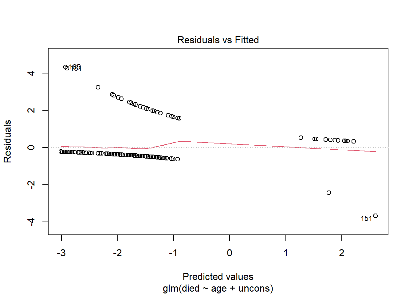
First let’s look at this plot for the original model fit to the subject-level data. We can do this by calling plot() on our model object and setting which = 1. Standardized Pearson residuals are plotted on the y-axis versus predicted log-odds on the x-axis. This produces strange, uninformative, somewhat parallel lines. There’s not much we can infer from this plot.
plot(m, which = 1)

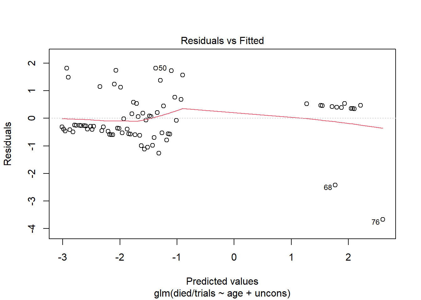
Now create the same plot using the model fit to the group-level data. This plot is more informative and looks similar to the type of Residuals vs. Fitted plot we see evaluating linear models.
plot(m2, which = 1)

As usual, we want to see that we’re not systematically over- or under-predicting. It appears at the lower predicted values, we’re under-fitting a bit. The observed proportions are larger than the predicted proportions. At the higher predicted values, we're over-fitting for a couple of predictor patterns. The observed proportions are much smaller than the predicted proportions.
The labeled points refer to rows in our data. We can use those to investigate the residuals. For example, looking at rows 68 and 76, we see that our model predicts high probability of dying, but these subjects lived. Thus we have large residuals. But also notice each prediction is based on one observation. We should be cautious reading too much into these residuals. Even though this model is based on group-level data, we still have instances of groups with just one observation.
ICU_grp$pred <- predict(m2, type = "response")
ICU_grp$deviance <- residuals(m2)
ICU_grp[c(68, 76),]
     age uncons died trials proportion      pred  deviance
  68  59    Yes    0      1          0 0.8543873 -1.963061
  76  89    Yes    0      1          0 0.9310534 -2.312757
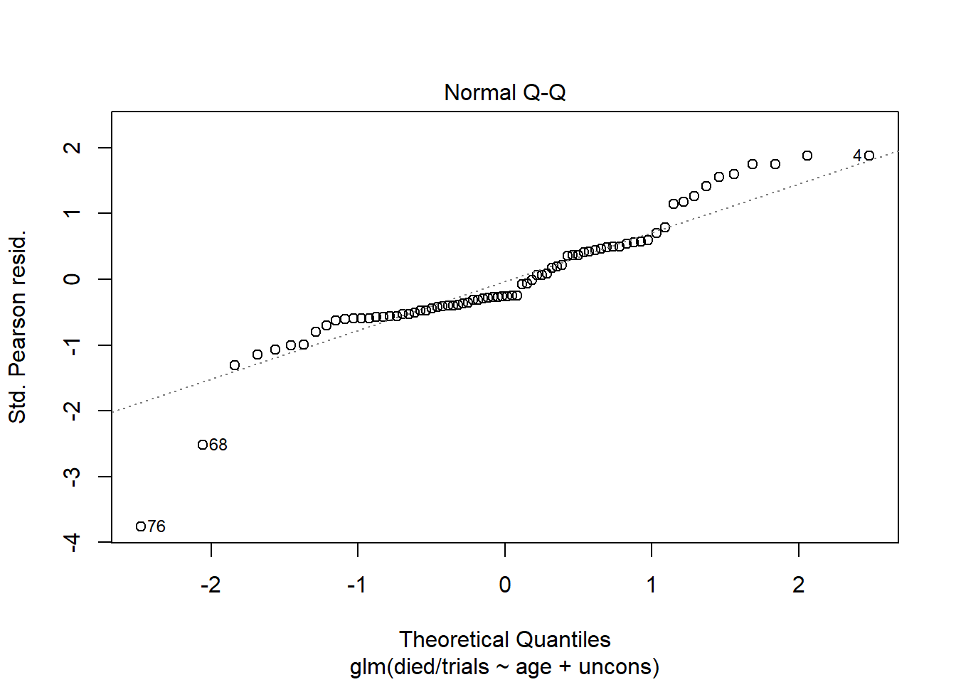
Earlier we mentioned that standardized Pearson residuals have an approximate standard normal distribution if the model fits. This implies looking at a QQ Plot of residuals can provide some assessment of model fit. We can produce this plot using plot() with which = 2. Again the plot created with the group-level model is more informative than the plot created with the subject-level model.
plot(m2, which = 2)

This suggests our model is holding well in the middle range of predicted values but is maybe suspect in the extremities. It’s worth mentioning that binomial logistic regression models have no error term or normality assumptions. In a standard linear model, this plot assesses normality of residuals, which is one of the assumptions of a linear model. But in a binary logistic regression model, normality of residuals is simply evidence of a decent fitting model. There is no assumption that residuals are random draws from a normal distribution.
We hope you now have a better understanding of deviance and Pearson residuals, how to interpret them, and when they’re most useful. Ideally, we like to work with them when a model is based on group-level data, but with many continuous predictors, group-level data may not be possible or result in too many unique predictor combinations.
R session details
The analysis was done using the R Statistical language (v4.5.1; R Core Team, 2025) on Windows 11 x64, using the packages vcdExtra (v0.8.6), vcd (v1.4.13) and gnm (v1.1.5).
References
- Agresti, A. (2002). Categorical data analysis (2nd ed.). Wiley.
- Bilder, C., & Loughin, T (2015). Analysis of categorical data with R. CRC Press.
- Friendly, M., & Meyer, D. (2016). Discrete data analysis with R: Visualization and modeling techniques for categorical and count data. CRC Press.
- Friendly, M. (2022). vcdExtra: ‘vcd’ extensions and additions (Version 0.8-0). https://CRAN.R-project.org/package=vcdExtra
- Harrell, F. (2015). Regression modeling strategies (2nd ed.). Springer. http://hbiostat.org/rmsc/
- R Core Team. (2022). R: A language and environment for statistical computing. R Foundation for Statistical Computing. https://www.R-project.org/
- Wilks, S. (1938). The large-sample distribution of the likelihood ratio for testing composite hypotheses. Annals of Mathematical Statistics 9(1), 60--62. https://doi.org/10.1214/aoms/1177732360
Clay Ford
Statistical Research Consultant
University of Virginia Library
September 28, 2022
- We can also calculate standardized deviance residuals using
rstandard()andtype = "deviance". It, too, uses hat values to adjust the deviance residuals. ↩︎ - Technically, we should multiply by the number of combinations that could result in 3 heads and 2 tails (i.e., the binomial coefficient) to get the true joint probability, but it doesn’t matter in the context of maximum likelihood. ↩︎
- Degrees of freedom here is the number of observations minus the number of model coefficients. ↩︎
For questions or clarifications regarding this article, contact statlab@virginia.edu.
View the entire collection of UVA Library StatLab articles, or learn how to cite.
