
I’ve heard something frightening from practicing statisticians who frequently use mixed effects models. Sometimes when I ask them whether they produced a [semi]variogram to check the correlation structure they reply “what’s that?” -Frank Harrell
When it comes to statistical modeling, semivariograms help us visualize and assess correlation in residuals. We can use them for two different purposes: (1) to detect correlation and (2) to check if our model has adequately addressed correlation. We show examples of both in this article in the context of multilevel/mixed-effect models.
To begin, let’s simulate multilevel data with no correlated residuals using R. That is, we will generate data for several subjects and add random noise that is uncorrelated. Below we specify 300 subjects (N) and that each subject will have 8 observations (n). We create a variable called id to identify each subject and set it as a factor (i.e., categorical variable). Next we create a simple independent variable called x, which is just the numbers 1 through 8. Finally we use expand.grid() to create every combination of x and id and save the result to an object called d, which is a data frame.
N <- 300  # number of subjects
n <- 8    # number of obs per subject
id <- factor(1:N)
x <- 1:n
d <- expand.grid(x = x, id = id)
Now we simulate two different sources of random noise: (1) between subjects, z, and (2) within subjects, e. (The set.seed(1) code allows you to simulate the same data if you would like to follow along.) Both come from normal distributions with mean 0 and standard deviations of 0.7 and 0.3, respectively. We might think of the values 0.7 and 0.3 as the true random effect parameters.
set.seed(1)
z <- rnorm(N, mean = 0, sd = 0.7)
e <- rnorm(N * n, mean = 0, sd = 0.3)
And now we simulate a response variable we’ll call y. The z[d$id] syntax extracts each subject-specific noise value and adds it to the intercept. The within-subject noise is added at the end. The fixed portion of the formula is 0.1 + 1.2(x). We might think of the values 0.1 and 1.2 as the true fixed effect parameters.
d$y <- (0.1 + z[d$id]) + 1.2 * d$x + e
If we wanted to “work backwards” and recover the true parameters, we could use the lmer() function in the lme4 package. Below we specify that y is a function of x with an intercept that is conditional on id. The summary reports parameter estimates for random and fixed effects. Notice the estimates are close to the true values we used to simulate the data. For example, the estimated standard deviation for the id random effect is 0.66, which is close to 0.7.
# install.packages("lme4")
library(lme4)
m_lmer <- lmer(y ~ x + (1 | id), data = d)
summary(m_lmer, corr = FALSE)
Linear mixed model fit by REML ['lmerMod']
Formula: y ~ x + (1 | id)
   Data: d
REML criterion at convergence: 2299.6
Scaled residuals:
    Min      1Q  Median      3Q     Max
-3.4810 -0.6263 -0.0185  0.6173  3.6365
Random effects:
 Groups   Name        Variance Std.Dev.
 id       (Intercept) 0.43659  0.6607
 Residual             0.09664  0.3109
Number of obs: 2400, groups:  id, 300
Fixed effects:
            Estimate Std. Error t value
(Intercept) 0.123609   0.040631   3.042
x           1.198760   0.002769 432.858
Another function we can use is the lme() function in the nlme package. This package is one of the recommended packages that comes installed with R. The main difference in the syntax is that we use random = ~ 1 | id to specify the random intercept. We leave it to the reader to verify that the results are identical. We also note that the "Correlation" estimate in the output has nothing to do with the topic of this article! See the following StatLab Article to learn more about interpreting correlation of fixed effects: https://library.virginia.edu/data/articles/correlation-of-fixed-effects-in-lme4
library(nlme)
m_lme <- lme(y ~ x, random = ~ 1 | id, data = d)
summary(m_lme)
Linear mixed-effects model fit by REML
  Data: d
       AIC      BIC    logLik
  2307.641 2330.771 -1149.821
Random effects:
 Formula: ~1 | id
        (Intercept)  Residual
StdDev:    0.660747 0.3108653
Fixed effects:  y ~ x
                Value  Std.Error   DF  t-value p-value
(Intercept) 0.1236087 0.04063083 2099   3.0422  0.0024
x           1.1987597 0.00276941 2099 432.8577  0.0000
 Correlation:
  (Intr)
x -0.307
Standardized Within-Group Residuals:
        Min          Q1         Med          Q3         Max
-3.48103043 -0.62627396 -0.01853078  0.61732176  3.63647704
Number of Observations: 2400
Number of Groups: 300
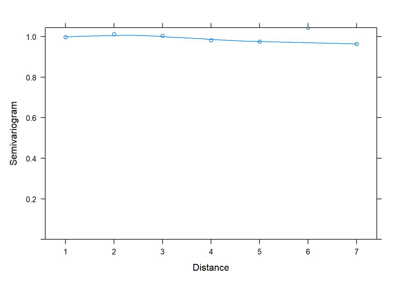
One reason we might want to use the lme() function in the nlme package is the built-in support for creating semivariograms. Below we use the plot() and Variogram() functions to create a semivariogram for our model residuals. Notice we specify the grouping structure in our data using the argument form = ~ 1 | id. The resulting plot shows points and a smooth almost-horizontal line around 1. This indicates there is no correlation in our model residuals.
plot(Variogram(m_lme, form = ~ 1 | id))
We will talk about how semivariograms are created shortly. But first let’s simulate data with correlated residuals and see what kind of semivariogram we get. Below we create a correlation matrix called ar1 using the toeplitz() function. We set phi equal to 0.8 and raise it to powers ranging from 0 to 7 using the code phi^(0:(n-1)). (Recall we defined n = 8 above, so n - 1 = 7.) The result is sometimes referred to as an “AR(1)” matrix, or autoregressive lag 1 matrix. Notice phi (0.8) is the correlation between two adjacent measures; phi^2 (0.64) is the correlation between measures 2 units apart, phi^3 (0.512) is the correlation between measures 3 units apart, and so on.
phi <- 0.8
ar1 <- toeplitz(phi^(0:(n-1)))
ar1
          [,1]     [,2]    [,3]   [,4]   [,5]    [,6]     [,7]      [,8]
[1,] 1.0000000 0.800000 0.64000 0.5120 0.4096 0.32768 0.262144 0.2097152
[2,] 0.8000000 1.000000 0.80000 0.6400 0.5120 0.40960 0.327680 0.2621440
[3,] 0.6400000 0.800000 1.00000 0.8000 0.6400 0.51200 0.409600 0.3276800
[4,] 0.5120000 0.640000 0.80000 1.0000 0.8000 0.64000 0.512000 0.4096000
[5,] 0.4096000 0.512000 0.64000 0.8000 1.0000 0.80000 0.640000 0.5120000
[6,] 0.3276800 0.409600 0.51200 0.6400 0.8000 1.00000 0.800000 0.6400000
[7,] 0.2621440 0.327680 0.40960 0.5120 0.6400 0.80000 1.000000 0.8000000
[8,] 0.2097152 0.262144 0.32768 0.4096 0.5120 0.64000 0.800000 1.0000000
Now we use our ar1 correlation matrix to simulate random noise with correlation. To do this we use the mvrnorm() function from the MASS package, which simulates data from a multivariate normal distribution. The argument mu = rep(0, n) says we want the means of our multivariate normal distribution to be all zeroes. The Sigma = ar1 argument specifies the correlation matrix we want to use to simulate the data. Notice we simulate N sets of multivariate normal data. This results in a matrix that is 300 rows by 8 columns. That’s 300 sets of 8 correlated random noise values for our 300 subjects. Notice we multiply the random noise by a parameter called sigma, which we set to 0.5. Finally we generate our response, y2, the same way as before, but this time we only have one source of noise, e2. In order to add the noise, we need to transpose the matrix using the t() function and then convert it to a vector using the c() function: c(t(e2))
sigma <- 0.5
set.seed(2)
e2 <- sigma * MASS::mvrnorm(n = N, mu = rep(0, n), Sigma = ar1)
d$y2 <- 0.1 + 1.2 * d$x + c(t(e2))
How can we work backwards to recover our true parameter estimates using the correct model? In this case we can use the gls() function from the nlme package. The gls() function fits a linear model using generalized least squares. This allows us to model correlated residuals. Below we specify correlation = corAR1(form = ~ 1 | id), which says the correlation model we want to fit is an AR1 model grouped by id. The corAR1() function is part of the nlme package. Notice in the summary output that the parameter estimate for "Phi" is 0.806, which is very close to our true phi value of 0.8. Notice also the residual standard error estimate of 0.511 is close to our true sigma value of 0.5.
m_gls <- gls(y2 ~ x, data = d, correlation = corAR1(form = ~ 1 | id))
summary(m_gls)
Generalized least squares fit by REML
  Model: y2 ~ x
  Data: d
      AIC     BIC    logLik
  1411.72 1434.85 -701.8602
Correlation Structure: AR(1)
 Formula: ~1 | id
 Parameter estimate(s):
      Phi
0.8061877
Coefficients:
                Value  Std.Error   t-value p-value
(Intercept) 0.1378911 0.03253754   4.23791       0
x           1.1890020 0.00525933 226.07495       0
 Correlation:
  (Intr)
x -0.727
Standardized residuals:
       Min         Q1        Med         Q3        Max
-3.4169056 -0.6816466 -0.0136351  0.6801660  3.0823354
Residual standard error: 0.5117779
Degrees of freedom: 2400 total; 2398 residual
And now back to semivariograms! We can use the plot() and Variogram() functions to assess correlation in residuals. Once again we specify form = ~ 1 | id since we have residuals grouped by id. Notice in the plot below we see an upward trend. This is evidence we have correlated residuals.
plot(Variogram(m_gls, form = ~ 1 | id))
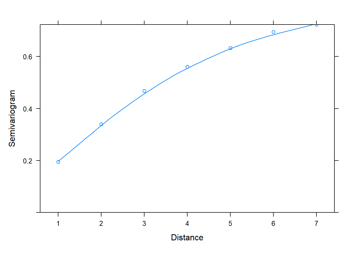
The x-axis is labeled “Distance”. This is the distance between residuals. Distance = 1 is for residuals that are adjacent, or next to each other. The "Semivariogram" value is 0.2. This is small relative to the Semivariogram value at Distance = 2, which appears to be a little higher than 0.3. This is for residuals 2 units apart. At Distance = 3, the Semivariogram value creeps up to about 0.5. This is for residuals 3 units apart. As the residuals get further apart, the Semivariogram value increases, which indicates residuals are getting further apart. This implies correlation between residuals shrinks as they get further apart in time.
If we add the argument resType = "normalized" to the Variogram() function, we get a different looking plot with a smooth almost-horizontal line at 1. This is evidence that our model adequately models the correlated residuals.
plot(Variogram(m_gls, form = ~ 1 | id, resType = "normalized"))
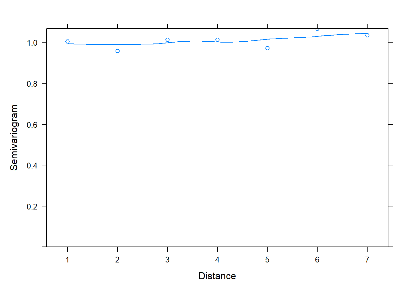
The resType = "normalized" argument says to plot normalized residuals. Technically speaking, these are standardized residuals pre-multiplied by the inverse square-root factor of the estimated error correlation matrix. That’s a mouthful, and the details are in Pinheiro and Bates (2000). But the important point is that if the within-group correlation model is correct, the normalized residuals should have an approximate standard normal distribution with mean 0 and standard deviation 1. Hence the points hovering around 1 in the semivariogram for an adequate model.
So how are semivariograms calculated? The basic idea is to take the difference between all possible pairs of residuals, square them, and divide by 2. The result is called the “semivariogram.”
\[\text{semivariogram} = (x - y)^2/2 \]
Let’s work through a toy example. Below we generate 5 uncorrelated residuals from a standard normal distribution and call the vector r. (It doesn’t matter whether the values are correlated or not for the purpose of this example.)
set.seed(3)
r <- rnorm(5)
r
[1] -0.9619334 -0.2925257 0.2587882 -1.1521319 0.1957828
Next we take the difference between all pairs of residuals, square the difference, and divide by 2. We can make quick work of this using the outer() function. Notice the result is a symmetric matrix. In row 1, the value 0.2240533 is the semivariogram value for the 1st and 2nd residuals. The next value, 0.74508065, is the semivariogram value for the 1st and 3rd residuals. And so on. Since the matrix is symmetric, the values in the first row are the mirror image of the values in the first column.
sv <- outer(r, r, function(x, y) ((x - y)^2)/2)
sv
           [,1]      [,2]       [,3]       [,4]       [,5]
[1,] 0.00000000 0.2240533 0.74508065 0.01808773 0.67015345
[2,] 0.22405333 0.0000000 0.15197353 0.36946138 0.11922262
[3,] 0.74508065 0.1519735 0.00000000 0.99534777 0.00198484
[4,] 0.01808773 0.3694614 0.99534777 0.00000000 0.90843704
[5,] 0.67015345 0.1192226 0.00198484 0.90843704 0.00000000
We only need one set of semivariogram values from the symmetric matrix we calculated, so we extract just the lower portion using the code sv[lower.tri(sv)] and save it as variog.
sv <- outer(r, r, function(x, y) ((x - y)^2)/2)
variog <- sv[lower.tri(sv)]
variog
 [1] 0.22405333 0.74508065 0.01808773 0.67015345 0.15197353 0.36946138
 [7] 0.11922262 0.99534777 0.00198484 0.90843704
Next we create a vector of “distances” between residuals. This is made easy with the dist() function. The result is the lower portion of a symmetric matrix containing the distances between residuals. This basically amounts to subtraction. The distance between 2 and 1 is 1. The distance between 5 and 3 is 2. And so on.
distance <- dist(x = 1:5)
distance
  1 2 3 4
2 1
3 2 1
4 3 2 1
5 4 3 2 1
Now we use the as.numeric() function to extract the distance values into a vector and display our variog and distance values as a data frame.
data.frame(variog, distance = as.numeric(distance))
       variog distance
1  0.22405333        1
2  0.74508065        2
3  0.01808773        3
4  0.67015345        4
5  0.15197353        1
6  0.36946138        2
7  0.11922262        3
8  0.99534777        1
9  0.00198484        2
10 0.90843704        1
We can get the same result using the Variogram() function from the nlme package.
Variogram(object = r, distance = dist(1:5))
       variog dist
1  0.22405333    1
2  0.74508065    2
3  0.01808773    3
4  0.67015345    4
5  0.15197353    1
6  0.36946138    2
7  0.11922262    3
8  0.99534777    1
9  0.00198484    2
10 0.90843704    1
Notice in the output we have four pairs of residuals with dist = 1. This refers to residual pairs (1,2), (2,3), (3,4), and (4,5). That is, we have 4 pairs of residuals that are next to each other, or one unit apart. We only have one value for dist = 4. That’s the semivariogram value for the residual pair (1,5).
If we run the Variogram() function on our fitted model, m_gls, we get a data frame with 7 rows and an extra column titled n.pairs. Since we generated 8 observations per subject, we have distances of 1 through 7 to consider. The n.pairs column refers to the number of pairs of residuals we have for each distance. The variog value is the mean semivariogram value for all 300 subjects.
Variogram(m_gls)
     variog dist n.pairs
1 0.1947631    1    2100
2 0.3397939    2    1800
3 0.4677898    3    1500
4 0.5606810    4    1200
5 0.6327643    5     900
6 0.6947439    6     600
7 0.7230897    7     300
We can manually calculate the variog values by splitting the Pearson residuals of our model by id, applying the Variogram() function to all sets, combining the result into a data frame, and calculating the mean variog value by dist.
r_mod <- residuals(m_gls, type = "pearson")
r_lst <- split(r_mod, d$id)
r_variog <- lapply(r_lst, function(x)Variogram(x, dist = dist(1:8)))
r_df <- do.call("rbind", r_variog)
aggregate(variog ~ dist, r_df, mean)
  dist    variog
1    1 0.1947631
2    2 0.3397939
3    3 0.4677898
4    4 0.5606810
5    5 0.6327643
6    6 0.6947439
7    7 0.7230897
And if we use the table() function on the dist column of our data frame, we reproduce the number of pairs.
table(r_df$dist)
   1    2    3    4    5    6    7
2100 1800 1500 1200  900  600  300
Creating semivariograms for models fit with nlme is convenient thanks to the built-in Variogram() and plot() methods. If we wanted to assess correlation in residuals after fitting a model using lme4, we would need to do it manually using code similar to what we used above. For example, let’s fit our model with correlated errors using a random-intercept model via lmer(). (Note this model assumes independent errors!)
# recall: y2 has correlated errors
m <- lmer(y2 ~ x + (1|id), data = d)
Now we calculate our semivariogram values manually using our code from above.
r_mod <- residuals(m)
r_lst <- split(r_mod, d$id)
r_variog <- lapply(r_lst, function(x)Variogram(x, dist = dist(1:8)))
r_df <- do.call("rbind", r_variog)
var_df <- aggregate(variog ~ dist, r_df, mean)
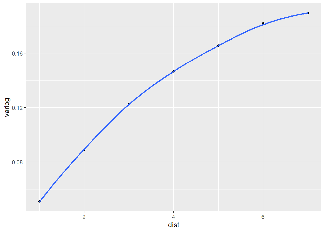
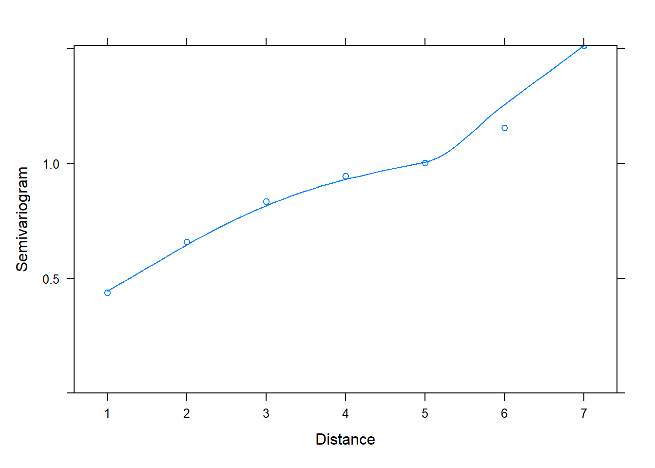
And finally we create our semivariogram plot using the ggplot2 package. The evidence of correlated residuals is overwhelming. This tells us the current model may not be adequate and that we may want to consider modeling the correlation structure of the residuals using either the gls() or lme() functions in the nlme package.
library(ggplot2)
ggplot(var_df) +
  aes(x = dist, y = variog) +
  geom_point() +
  geom_smooth(se = F)
The nlme package provides several functions for modeling serial and spatial correlation in residuals. Two simple ones for serial correlation are the corCompSymm() and corSymm() functions . The corCompSymm() function models all correlations between residuals as a single correlation parameter. For example, if phi = 0.8, that’s the estimated correlation between two residuals no matter how close or far apart they are in time. This is usually too simple. The corSymm() function models all correlations between residuals individually. For our current model, that would estimate (8 * 7)/2 = 28 separate correlation parameters. This is usually too complicated. The autoregressive lag 1 model we used above is usually a nice compromise.
Using a method described in Harrell (2015), we can try all three methods out and compare the models. Below we save the three functions into a list named cp and create an empty list called z the same length as cp. We then fit three models in a for loop, trying a different correlation structure each time. The models are then compared with the anova() function.
cp <- list(corCompSymm, corAR1, corSymm)
z  <- vector(mode = 'list',length = length(cp))
for(k in 1:length(cp)) {
  z[[k]] <- gls(y2 ~ x, data = d,
                correlation=cp[[k]](form = ~ 1 | id))
}
anova(z[[1]],z[[2]],z[[3]])
       Model df      AIC      BIC     logLik   Test  L.Ratio p-value
z[[1]]     1  4 2334.206 2357.336 -1163.1032
z[[2]]     2  4 1411.720 1434.850  -701.8602
z[[3]]     3 31 1445.096 1624.350  -691.5480 2 vs 3 20.62453  0.8036
We see that all model statistics point to model 2, the corAR1() model, as the preferred model, which makes sense since the errors really were generated with an AR(1) correlation matrix. The last line also shows the results for a likelihood ratio test with a p-value of 0.8. The null hypothesis is that model 2 (the simpler model) is just as good as model 3 (the more complex model). Such a high p-value leads us to not reject this null hypothesis and to choose to retain the simpler model.
The first model, fit with corCompSymm(), does not seem to be an adequate model compared to models 2 and 3. In fact we can check the semivariogram plot of its normalized residuals to verify that it is not properly modeling correlation between residuals. We conclude this due to the positive increasing trendline of semivariogram values over distance.
plot(Variogram(z[[1]], form = ~ 1 |id, resType = "normalized"))
Hopefully you now have a better understanding of how to create and interpret semivariograms.
R session details
The analysis was done using the R Statistical language (v4.5.1; R Core Team, 2025) on Windows 11 x64, using the packages lme4 (v1.1.37), Matrix (v1.7.3), nlme (v3.1.168) and ggplot2 (v3.5.2).
References
- Bates, D., Maechler, M., Bolker, B., & Walker, S. (2015). Fitting linear mixed-effects models using lme4. Journal of Statistical Software, 67(1), 1--48. https://doi.org/10.18637/jss.v067.i01
- Harrell, F., Jr. (2015). Regression modeling strategies (2nd ed.). Springer. https://doi.org/10.1007/978-3-319-19425-7
- Pinheiro, J. C., & Bates, D. M. (2000). Mixed-effects models in S and S-PLUS. Springer. https://doi.org/10.1007/b98882.
- Pinheiro, J., Bates, D., & R Core Team. (2022). nlme: Linear and nonlinear mixed effects models (Version 3.1-160). https://CRAN.R-project.org/package=nlme.
- R Core Team. (2022). R: A language and environment for statistical computing. R Foundation for Statistical Computing. https://www.R-project.org/.
- Venables, W. N., & Ripley, B. D. (2002) Modern applied statistics with S (4th ed.). Springer. https://doi.org/10.1007/978-0-387-21706-2
- Wickham, H. (2016). ggplot2: Elegant graphics for data analysis. Springer-Verlag. https://doi.org/10.1007/978-3-319-24277-4
Clay Ford
Statistical Research Consultant
University of Virginia Library
December 14, 2022
For questions or clarifications regarding this article, contact statlab@virginia.edu.
View the entire collection of UVA Library StatLab articles, or learn how to cite.