
What are robust standard errors? How do we calculate them? Why use them? Why not use them all the time if they’re so robust? Those are the kinds of questions this post intends to address.
To begin, let’s start with the relatively easy part: getting robust standard errors for basic linear models in Stata and R. In Stata, simply appending vce(robust) to the end of regression syntax returns robust standard errors. “vce” is short for “variance-covariance matrix of the estimators.” “robust” indicates which type of variance-covariance matrix to calculate. Here’s a quick example using the auto data set that comes with Stata 16:
. sysuse auto
(1978 Automobile Data)
. regress mpg turn trunk, vce(robust)
Linear regression                               Number of obs     =         74
                                                F(2, 71)          =      68.76
                                                Prob > F          =     0.0000
                                                R-squared         =     0.5521
                                                Root MSE          =      3.926

------------------------------------------------------------------------------
             |               Robust
         mpg |      Coef.   Std. Err.      t    P>|t|     [95% Conf. Interval]
-------------+----------------------------------------------------------------
        turn |  -.7610113   .1447766    -5.26   0.000    -1.049688    -.472335
       trunk |  -.3161825   .1229278    -2.57   0.012    -.5612936   -.0710714
       _cons |   55.82001   4.866346    11.47   0.000     46.11679    65.52323
Notice the third column indicates “robust” standard errors.
To replicate the result in R takes a bit more work. First we load the haven package to use the read_dta() function that allows us to import Stata data sets. Then we load two more packages: lmtest and sandwich. The lmtest package provides the coeftest() function that allows us to re-calculate a coefficient table using a different variance-covariance matrix. The sandwich package provides the vcovHC() function that allows us to calculate robust standard errors. The type argument allows us to specify what kind of robust standard errors to calculate. “HC1” is one of several types available in the sandwich package and happens to be the default type in Stata 16. (We talk more about the different types and why it’s called the “sandwich” package below.)
library(haven)
library(lmtest)
library(sandwich)

auto <- read_dta('http://www.stata-press.com/data/r16/auto.dta')
m <- lm(mpg ~ turn + trunk, data = auto)
coeftest(m, vcov. = vcovHC(m, type = 'HC1'))
  t test of coefficients:

              Estimate Std. Error t value  Pr(>|t|)
  (Intercept) 55.82001    4.86635 11.4706 < 2.2e-16 ***
  turn        -0.76101    0.14478 -5.2565 1.477e-06 ***
  trunk       -0.31618    0.12293 -2.5721    0.0122 *
  ---
  Signif. codes:  0 '***' 0.001 '**' 0.01 '*' 0.05 '.' 0.1 ' ' 1
If you look carefully, you’ll notice the standard errors in the R output match those in the Stata output.
If we want 95% confidence intervals like those produced in Stata, we need to use the coefci() function:
coefci(m, vcov. = vcovHC(m, type = 'HC1'))
                   2.5 %      97.5 %
  (Intercept) 46.1167933 65.52322937
  turn        -1.0496876 -0.47233499
  trunk       -0.5612936 -0.07107136
While not really the point of this post, we should note the results say that larger turn circles and bigger trunks are associated with lower gas mileage.
Now that we know the basics of getting robust standard errors out of Stata and R, let’s talk a little about why they’re robust by exploring how they’re calculated.
The usual method for estimating coefficient standard errors of a linear model can be expressed with this somewhat intimidating formula:
$${Var}(\hat{\beta}) = (X^TX)^{-1} X^T\Omega X (X^TX)^{-1}$$
where \(X\) is the model matrix (i.e., the matrix of the predictor values) and \(\Omega = \sigma^2 I_n\), which is shorthand for a matrix with nothing but \(\sigma^2\) on the diagonal and 0’s everywhere else. Two main things to notice about this equation:
- The \(X^T \Omega X\) in the middle
- The \((X^TX)^{-1}\) on each side
Some statisticians and econometricians refer to this formula as a "sandwich" because it's like an equation sandwich: We have "meat" in the middle, \(X^T \Omega X\), and "bread" on the outside, \((X^TX)^{-1}\). Calculating robust standard errors means substituting a new kind of "meat."
Before we do that, let's use this formula by hand to see how it works when we calculate the usual standard errors. This will give us some insight to the meat of the sandwich. To make this easier to demonstrate, we'll use a small toy data set.
set.seed(1)
x <- c(1:4, 7)
y <- c(5 + rnorm(4,sd = 1.2), 35)
plot(x, y)
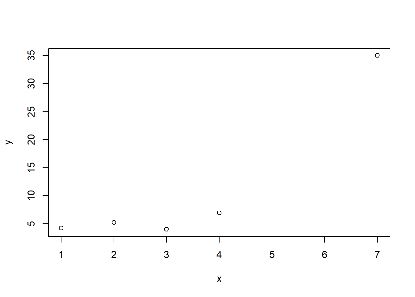
Notice the way we generated y. It is simply the number 5 with some random noise from a \(N(0,1.2)\) distribution plus the number 35. There is no relationship between x and y. However, when we regress y on x using lm() we get a slope coefficient of about 5.2 that appears to be “significant”.
m <- lm(y ~ x)
summary(m)
  Call:
  lm(formula = y ~ x)

  Residuals:
       1      2      3      4      5
   5.743  1.478 -4.984 -7.304  5.067

  Coefficients:
              Estimate Std. Error t value Pr(>|t|)
  (Intercept)   -6.733      5.877  -1.146   0.3350
  x              5.238      1.479   3.543   0.0383 *
  ---
  Signif. codes:  0 '***' 0.001 '**' 0.01 '*' 0.05 '.' 0.1 ' ' 1

  Residual standard error: 6.808 on 3 degrees of freedom
  Multiple R-squared:  0.8071, Adjusted R-squared:  0.7428
  F-statistic: 12.55 on 1 and 3 DF,  p-value: 0.03829
Clearly the 5th data point is highly influential and driving the “statistical significance,” which might lead us to think we have specified a “correct” model. Of course, we know that we specified a “wrong” model because we generated the data. y does not have a relationship with x! It would be nice if we could guard against this sort of thing from happening: specifying a wrong model but getting a statistically significant result. One way we could do that is modifying how the coefficient standard errors are calculated.
Let’s see how they were calculated in this case using the formula we specified above. Below s2 is \(\sigma^2\), diag(5) is \(I_n\), and X is the model matrix. Notice we can use the base R function model.matrix() to get the model matrix from a fitted model. We save the formula result into vce, which is the variance-covariance matrix. Finally we take square root of the diagonal elements to get the standard errors output in the model summary.
s2 <- sigma(m)^2
X <- model.matrix(m)
vce <- solve(t(X) %*% X) %*% (t(X) %*% (s2*diag(5)) %*% X) %*% solve(t(X) %*% X)
sqrt(diag(vce))
  (Intercept)           x
     5.877150    1.478557
Now let’s take a closer look at the “meat” in this sandwich formula:
s2*diag(5)
         [,1]   [,2]   [,3]   [,4]   [,5]
  [1,] 46.346  0.000  0.000  0.000  0.000
  [2,]  0.000 46.346  0.000  0.000  0.000
  [3,]  0.000  0.000 46.346  0.000  0.000
  [4,]  0.000  0.000  0.000 46.346  0.000
  [5,]  0.000  0.000  0.000  0.000 46.346
That is a matrix of constant variance. This is one of the assumptions of classic linear modeling: The errors (or residuals) are drawn from a single normal distribution with mean 0 and a fixed variance. The s2 object above is the estimated variance of that normal distribution. But what if we modified this matrix so that the variance was different for some observations? For example, it might make sense to assume the error of the 5th data point was drawn from a normal distribution with a larger variance. This would result in a larger standard error for the slope coefficient, indicating greater uncertainty in our coefficient estimate.
This is the idea of “robust” standard errors: modifying the “meat” in the sandwich formula to allow for things like non-constant variance (and/or autocorrelation, a phenomenon we don’t address in this post).
So how do we automatically determine non-constant variance estimates? It might not surprise you that there are several ways. The sandwich package provides seven different types at the time of this writing (version 2.5-1). The default version in Stata is identified in the sandwich package as “HC1”. The HC stands for heteroskedasticity-consistent. Heteroskedasticity is another word for non-constant. The formula for “HC1” is as follows:
$$HC1: \frac{n}{n-k}\hat{\mu}_i^2$$
where \(\hat{\mu}_i^2\) refers to squared residuals, \(n\) is the number of observations, and \(k\) is the number of coefficients. In our simple model above, \(k = 2\), since we have an intercept and a slope. Let’s modify our formula above to substitute HC1 “meat” in our sandwich:
# HC1
hc1 <- (5/3)*resid(m)^2

# HC1 "meat"
hc1*diag(5)
          [,1]     [,2]     [,3]     [,4]     [,5]
  [1,] 54.9775 0.000000  0.00000  0.00000  0.00000
  [2,]  0.0000 3.638417  0.00000  0.00000  0.00000
  [3,]  0.0000 0.000000 41.39379  0.00000  0.00000
  [4,]  0.0000 0.000000  0.00000 88.92616  0.00000
  [5,]  0.0000 0.000000  0.00000  0.00000 42.79414
Notice we no longer have constant variance for each observation. The estimated variance is instead the residual squared multiplied by (5/3). When we use this to estimate “robust” standard errors for our coefficients, we get slightly different estimates.
vce_hc1 <- solve(t(X) %*% X) %*% (t(X) %*% (hc1*diag(5)) %*% X) %*% solve(t(X) %*% X)
sqrt(diag(vce_hc1))
  (Intercept)           x
     5.422557    1.428436
Notice the slope standard error actually got smaller. It looks like the HC1 estimator may not be the best choice for such a small sample. The default estimator for the sandwich package is known as “HC3”:
$$HC3: \frac{\hat{\mu}_i^2}{(1 - h_i)^2}$$
where \(h_i\) are the hat values from the hat matrix. A Google search or any textbook on linear modeling can tell you more about hat values and how they’re calculated. For our purposes, it suffices to know that they range from 0 to 1, and that larger values are indicative of influential observations. We see then that HC3 is a ratio that will be larger for values with high residuals and relatively high hat values. We can manually calculate the HC3 estimator using the base R resid() and hatvalues() functions as follows:
# HC3
hc3 <- resid(m)^2/(1 - hatvalues(m))^2

# HC3 "meat"
hc3*diag(5)
           [,1]     [,2]     [,3]     [,4]     [,5]
  [1,] 118.1876 0.000000  0.00000  0.00000   0.0000
  [2,]   0.0000 4.360667  0.00000  0.00000   0.0000
  [3,]   0.0000 0.000000 39.54938  0.00000   0.0000
  [4,]   0.0000 0.000000  0.00000 87.02346   0.0000
  [5,]   0.0000 0.000000  0.00000  0.00000 721.2525
Notice that the 5th observation has a huge estimated variance of about 721. When we calculate the robust standard errors for the model coefficients we get a much bigger standard error for the slope.
vce_hc3 <- solve(t(X) %*% X) %*% (t(X) %*% (hc3*diag(5)) %*% X) %*% solve(t(X) %*% X)
sqrt(diag(vce_hc3))
  (Intercept)           x
    12.149991    4.734495
Of course we wouldn’t typically calculate robust standard errors by hand like this. We would use the vcovHC() function in the sandwich package as we demonstrated at the beginning of this post along with the coeftest() function from the lmtest package. (Or use vce(hc3) in Stata.)
coeftest(m, vcovHC(m, "HC3"))
  t test of coefficients:

              Estimate Std. Error t value Pr(>|t|)
  (Intercept)  -6.7331    12.1500 -0.5542   0.6181
  x             5.2380     4.7345  1.1063   0.3493
Now the slope coefficient estimate is no longer “significant” since the standard error is larger. This standard error estimate is robust to the influence of the outlying 5th observation.
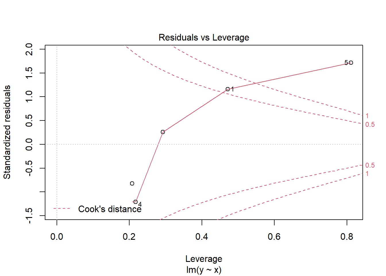
So when should we use robust standard errors? One flag is seeing large residuals and high leverage (i.e., hat values). For instance, the following base R diagnostic plot graphs residuals versus hat values. A point in the upper or lower right corners is an observation exhibiting influence on the model. Our 5th observation has a corner all to itself.
plot(m, which = 5)
But it’s important to remember large residuals (or evidence of non-constant variance) could be due to a misspecified model. We may be missing key predictors, interactions, or non-linear effects. Because of this, it might be a good idea to think carefully about your model before reflexively deploying robust standard errors. Zeileis (2006), the author of the sandwich package, also gives two reasons for not using robust standard errors “for every model in every analysis”:
First, the use of sandwich estimators when the model is correctly specified leads to a loss of power. Second, if the model is not correctly specified, the sandwich estimators are only useful if the parameters estimates are still consistent, i.e., if the misspecification does not result in bias.
We can demonstrate each of these points via simulation.
In the first simulation, we generate data with an interaction, fit the correct model, and then calculate both the usual and robust standard errors. We then check how often we correctly reject the null hypothesis of no interaction between x and g. This is an estimation of power for this particular hypothesis test.
# function to generate data, fit correct model, and extract p-values of
# interaction
f1 <- function(n = 50){
  # generate data
  g <- gl(n = 2, k = n/2)
  x <- rnorm(n, mean = 10, sd = 2)
  y <- 1.2 + 0.8*(g == "2") + 0.6*x + -0.5*x*(g == "2") + rnorm(n, sd = 1.1)
  d <- data.frame(y, g, x)
  # fit correct model
  m1 <- lm(y ~ g + x + g:x, data = d)
  sm1 <- summary(m1)
  sm2 <- coeftest(m1, vcov. = vcovHC(m1))
  # get p-values using usual SE and robust ES
  c(usual = sm1$coefficients[4,4],
    robust = sm2[4,4])
}

# run the function 1000 times
r_out <- replicate(n = 1000, expr = f1())

# get proportion of times we correctly reject Null of no interaction at p < 0.05
# (ie, estimate power)
apply(r_out, 1, function(x)mean(x < 0.05))
   usual robust
   0.835  0.789
The proportion of times we reject the null of no interaction using robust standard errors is lower than simply using the usual standard errors, which means we have a loss of power. (Though admittedly, the loss of power in this simulation is rather small.)
The second simulation is much like the first, except now we fit the wrong model and get biased estimates.
# generate data
g <- gl(n = 2, k = 25)
x <- rnorm(50, mean = 10, sd = 2)
y <- 0.2 + 1.8*(g == "2") + 1.6*x + -2.5*x*(g == "2") + rnorm(50, sd = 1.1)
d <- data.frame(y, g, x)

# fit the wrong model: a polynomial in x without an interaction with g
m1 <- lm(y ~ poly(x, 2), data = d)

# use the wrong model to simulate 50 sets of data
sim1 <- simulate(m1, nsim = 50)

# plot a density curve of the original data
plot(density(d$y))

# overlay estimates from the wrong model
for(i in 1:50)lines(density(sim1[[i]]), col = "grey80")
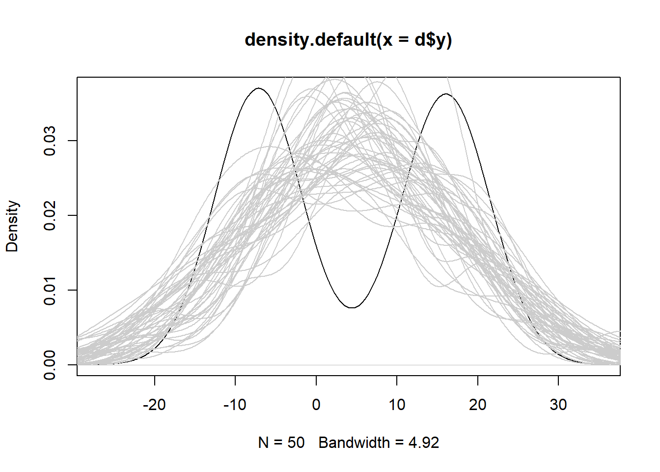
We see the simulated data from the wrong model is severely biased and is consistently over- or under-estimating the response. In this case robust standard errors would not be useful because our model is wrong.
Related to this last point, Freedman (2006) expresses skepticism about even using robust standard errors:
If the model is nearly correct, so are the usual standard errors, and robustification is unlikely to help much. On the other hand, if the model is seriously in error, the sandwich may help on the variance side, but the parameters being estimated…are likely to be meaningless---except perhaps as descriptive statistics.
There is much to think about before using robust standard errors. But hopefully you now have a better understanding of what they are and how they’re calculated. Zeileis (2004) provides a deeper and accessible introduction to the sandwich package, including how to use robust standard errors for addressing suspected autocorrelation.
R session details
The analysis was done using the R Statistical language (v4.5.1; R Core Team, 2025) on Windows 11 x64, using the packages haven (v2.5.5), zoo (v1.8.14), lmtest (v0.9.40) and sandwich (v3.1.1).
References
- Freedman, D. A. (2006). On the so-called "Huber sandwich estimator" and "robust standard errors." The American Statistician, 60(4). 299--302.
- R Core Team. (2020). R: A language and environment for statistical computing. R Foundation for Statistical Computing. URL https://www.R-project.org/
- StataCorp. (2019). Stata statistical software (Version 16). StataCorp LLC.
- StataCorp. (2019). Stata 16 base reference manual. Stata Press.
- Zeileis, A., & Hothorn, T. (2002). Diagnostic checking in regression relationships. R News, 2(3), 7--10. https://cran.r-project.org/doc/Rnews/Rnews_2002-3.pdf
- Zeileis, A. (2004). Econometric computing with HC and HAC covariance matrix estimators. Journal of Statistical Software, 11(10), 1--17. https://doi.org/10.18637/jss.v011.i10
- Zeileis, A. (2006). Object-oriented computation of sandwich estimators. Journal of Statistical Software, 16(9), 1--16. https://doi.org/10.18637/jss.v016.i09
Clay Ford
Statistical Research Consultant
University of Virginia Library
September 27, 2020
For questions or clarifications regarding this article, contact statlab@virginia.edu.
View the entire collection of UVA Library StatLab articles, or learn how to cite.