
Logistic regression is a method for modeling binary data as a function of other variables. For example we might want to model the occurrence or non-occurrence of a disease given predictors such as age, race, weight, etc. The result is a model that returns a predicted probability of occurrence (or non-occurrence, depending on how we set up our data) given certain values of our predictors. We might also be able to interpret the coefficients in our model to summarize how a change in one predictor affects the odds of occurrence. Logistic regression is a mature and effective statistical method used in many fields of study. A quick web search should yield many tutorials for getting started with logistic regression. The topic of this blog post is simulating binary data using a logistic regression model.
Using the sample() function we can easily simulate binary data with specified probabilities. Here’s a sample of 20 zeroes and ones, where 0 has a 30% chance of being sampled and 1 has a 70% chance of being sampled.
sample(c(0,1), size = 20, replace = TRUE, prob = c(0.3, 0.7))
[1] 1 1 1 0 0 0 1 0 1 1 1 1 1 1 1 1 1 0 1 1
Another way is to use the rbinom() function, which generates random values from a binomial distribution with a certain trial size and probability p of success or occurrence. To generate similar data as we did with sample(), set n = 20 to indicate 20 draws from a binomial distribution, set size = 1 to indicate the distribution is for 1 trial, and p = 0.7 to specify the distribution is for a “success” probability of 0.7:
rbinom(n = 20, size = 1, prob = 0.7)
[1] 0 0 1 1 1 1 1 1 1 1 1 1 0 1 0 1 0 0 0 1
It may help to think of the binomial distribution as the “coin flipping distribution”. Above 20 people flipped a coin 1 time that was loaded to land heads (or tails as the case may be) 70% percent of the time. If we wanted we could simulate 10 people each flipping 5 fair coins and see how many heads they get:
rbinom(n = 10, size = 5, prob = 0.5)
[1] 2 3 1 3 4 1 3 4 4 3
The result is the number of heads each person observed. But in this article, we’re concerned with binary data, so we’ll stick to results of 0 and 1 (i.e., size = 1).
Now we may want to simulate binary data where the probability changes conditional on other variables. For example, we might want the probability of a “1” for a 50-year-old male to be higher than the probability of a “1” for a 35-year-old male, which we might want higher than the probability of a “1” for a 35-year-old female. What we want is a model where we can plug in values such as age and gender and generate probabilities for churning out ones and zeroes. This is what a logistic regression model allows us to do.
Here’s the general logistic regression model:
\[Prob\{Y = 1|X\} = \frac{1}{1 + \text{exp}(-X\beta)}\]
The \(X\) represents our predictors. The \(\beta\) represents weights or coefficients for our predictors. If we had two predictors, \(X_1\) and \(X_2\), then \(X\beta = X_1\beta_1 + X_2\beta_2\). No matter what we plug into the model, it always returns a value between 0 and 1, or a probability. It’s easy to demonstrate with a quick plot.
x <- seq(-4, 4, length.out = 100)
p <- 1/(1 + exp(-x))
plot(x, p, type = "l")
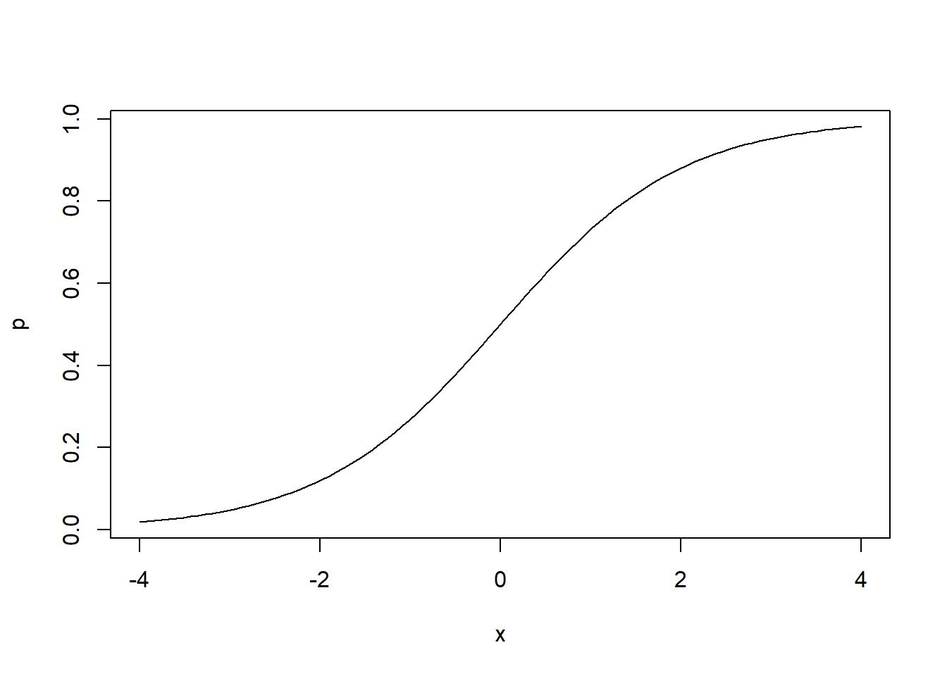
No matter our x value, p is bounded between 0 and 1.
Let’s use \(X\beta\) to generate some probabilities. Assume we have two predictors: gender and age. Gender is 1 for male, 0 for female. Age can take values from 18 to 80. Here’s one way to simulate those variables using the sample() and runif() functions. The sample() function samples from the vector c(0,1) with replacement 100 times. The runif() function draws 100 values from a uniform distribution that ranges in value from 18 to 80. If you run the set.seed(1) line of code, you will generate the same “random” values as we did.
set.seed(1)
gender <- sample(c(0,1), size = 100, replace = TRUE)
age <- round(runif(100, 18, 80))
Now let’s pick some values for \(\beta\). The \(\beta\) values represent the change in log odds per unit change in the predictors. If that sounds confusing, that’s completely normal. We talk a bit more about how to make sense of these values a little further down. For now let’s just pick some \(\beta\) values. Notice we’ve included an intercept.
xb <- -9 + 3.5*gender + 0.2*age
Now we can generate some probabilities using the logistic regression model:
p <- 1/(1 + exp(-xb))
summary(p)
    Min.  1st Qu.   Median     Mean  3rd Qu.     Max.
0.006693 0.354344 0.953552 0.721658 0.996816 0.999966
Notice p lies between 0 and 1, as probabilities should. Finally, with our probabilities we can generate ones and zeroes to indicate occurrence and non-occurrence using the rbinom() function:
set.seed(2)
y <- rbinom(n = 100, size = 1, prob = p)
y
  [1] 1 1 0 1 1 1 0 0 1 1 1 1 1 0 0 1 1 0 1 1 1 1 0 0 1 1 1 0 1 1 1 0 0 1 1 1 1
 [38] 1 1 1 1 1 0 1 1 1 0 1 0 1 1 1 1 1 1 0 1 1 1 0 0 1 1 1 1 1 0 0 1 1 1 1 1 0
 [75] 0 1 1 1 1 1 1 0 1 1 1 0 1 1 1 1 0 0 0 1 0 1 0 1 1 1
Let’s run a logistic regression on our data and see how well it recovers the “true” \(\beta\) values of -9, 3.5, and 0.2. For this we use the glm() function with family = "binomial":
mod <- glm(y ~ gender + age, family = "binomial")
summary(mod)
Call:
glm(formula = y ~ gender + age, family = "binomial")

Coefficients:
            Estimate Std. Error z value Pr(>|z|)
(Intercept) -7.73471    1.75431  -4.409 1.04e-05 ***
gender       2.97831    0.87401   3.408 0.000655 ***
age          0.17251    0.03784   4.559 5.14e-06 ***
---
Signif. codes:  0 '***' 0.001 '**' 0.01 '*' 0.05 '.' 0.1 ' ' 1

(Dispersion parameter for binomial family taken to be 1)

    Null deviance: 118.591  on 99  degrees of freedom
Residual deviance:  53.055  on 97  degrees of freedom
AIC: 59.055

Number of Fisher Scoring iterations: 7
The regression worked ok it appears. The true values are within 2 standard errors of the estimated coefficients. We can verify this by calculating 95% confidence intervals on the coefficients.
confint(mod)
                 2.5 %     97.5 %
(Intercept) -11.786616 -4.7725523
gender        1.441938  4.9409354
age           0.109164  0.2601939
Increasing the sample size from 100 to 1000 improves the estimation.
set.seed(111)
gender <- sample(c(0,1), size = 1000, replace = TRUE)
age <- round(runif(1000, 18, 80))
xb <- -9 + 3.5*gender + 0.2*age
p <- 1/(1 + exp(-xb))
y <- rbinom(n = 1000, size = 1, prob = p)
mod <- glm(y ~ gender + age, family = "binomial")
confint(mod)
                  2.5 %     97.5 %
(Intercept) -11.0542193 -8.2408681
gender        3.1118927  4.4321987
age           0.1801364  0.2394004
Let’s return to the coefficients we selected. We set the gender coefficient to 3.5. Recall that these values represent change in log odds. So when gender = 1 (male), the log odds increase by 3.5. That’s not intuitive. Fortunately we can exponentiate the coefficient to express it in terms of an odds ratio. Let’s do that:
exp(3.5)
[1] 33.11545
This says the odds of a “1” for a male are about 33 times the odds of a “1” for a female. This is a little easier to grasp. If the “1” means disease occurrence, this means the odds of a male contracting the disease are 33 times higher than the odds of a female contracting the disease. To express this in terms of a probability we would need to actually use our model to get predicted probabilities. Our model includes age, so let’s set age to 30 and compare the probability of disease between a 30-year-old male and a 30-year-old female. Again we use the general logistic regression model:
# male, age 30
p_male <- 1/(1 + exp(-(-9 + 3.5*1 + 0.2*30)))
p_male
[1] 0.6224593
# female, age 30
p_female <- 1/(1 + exp(-(-9 + 3.5*0 + 0.2*30)))
p_female
[1] 0.04742587
0.62 versus about 0.05. We can express that as an odds ratio as follows:
(0.62/(1 - 0.62))/(0.047/(1 - 0.047))
[1] 33.08287
Which is close to what we got by simply exponentiating the coefficient. Try the preceding calculations with different ages and you’ll notice you always get an odds ratio of about 33.
We can do the same with the age coefficient.
exp(0.2)
[1] 1.221403
This says the odds of occurrence increase by about 1.22 for each year someone gets older. Sometimes people will say the odds increase by about 22% since multiplying a quantity times 1.22 returns the quantity increased by 22%.
What about the intercept? Why include it? To see why, let’s simulate the data without it and then create a cross-tabulated table to see how occurrences break down across age and gender. Notice we use the cut() function to quickly create 4 arbitrary age groups containing equal numbers of people. This is simply to help create the table.
set.seed(2)
gender <- sample(c(0,1), size = 100, replace = TRUE)
age <- round(runif(100, 18, 80))
xb <- 3.5*gender + 0.2*age
p <- 1/(1 + exp(-xb))
y <- rbinom(n = 100, size = 1, prob = p)
xtabs(~ cut(age,4) + gender + y)
, , y = 1

           gender
cut(age, 4)  0  1
  (18.9,34] 17 14
  (34,49]   15  9
  (49,64]    6 11
  (64,79.1] 11 17
The result of our simulated data is that everyone got a “1” (occurrence)! It’s no wonder. Look at how high all the probabilities are:
summary(p)
   Min. 1st Qu.  Median    Mean 3rd Qu.    Max.
 0.9781  0.9995  1.0000  0.9987  1.0000  1.0000
Adding an intercept can help spread out the probabilities. It takes some trial and error. Let’s try adding -9.
set.seed(2)
xb <- -9 + 3.5*gender + 0.2*age
p <- 1/(1 + exp(-xb))
y <- rbinom(n = 100, size = 1, prob = p)
xtabs(~ cut(age,4) + gender + y)
, , y = 0

           gender
cut(age, 4)  0  1
  (18.9,34] 15 10
  (34,49]   11  1
  (49,64]    1  0
  (64,79.1]  0  0

, , y = 1

           gender
cut(age, 4)  0  1
  (18.9,34]  2  4
  (34,49]    4  8
  (49,64]    5 11
  (64,79.1] 11 17
That’s a little better. Now we’re seeing some non-occurrences. Remember, our plan is to use age as a numeric predictor, not categorical, so the 0 entries in the higher age groups may not bother us. If we want the balance of 0’s and 1’s spread out we could continue to play around with the intercept.
It’s important to note that the intercept in this example produces the predicted probability of a female (gender = 0) at age = 0. That may not be meaningful (unless we’re dealing with an event that could occur at birth). If we wanted, we could center the age variable by subtracting the mean age from each value. That means an age of 0 represents the mean age. In that case the intercept would produce the predicted probability for a female at the mean age. Let’s try that approach without specifying an intercept. Notice we use the scale() function on-the-fly to quickly center the age variable:
xb <- 3.5*gender + 0.2*scale(age, center = TRUE, scale = FALSE)
p <- 1/(1 + exp(-xb))
y <- rbinom(n = 100, size = 1, prob = p)
xtabs(~ cut(age,4) + gender + y)
, , y = 0

           gender
cut(age, 4)  0  1
  (18.9,34] 17 14
  (34,49]   14  0
  (49,64]    0  0
  (64,79.1]  0  0

, , y = 1

           gender
cut(age, 4)  0  1
  (18.9,34]  0  0
  (34,49]    1  9
  (49,64]    6 11
  (64,79.1] 11 17
That produces a decent spread of occurrences over gender and age. Let’s see what adding an intercept of -3 does:
xb <- -3 + 3.5*gender + 0.2*scale(age, center = TRUE, scale = FALSE)
p <- 1/(1 + exp(-xb))
y <- rbinom(n = 100, size = 1, prob = p)
xtabs(~ cut(age,4) + gender + y)
, , y = 0

           gender
cut(age, 4)  0  1
  (18.9,34] 17 14
  (34,49]   15  4
  (49,64]    4  1
  (64,79.1]  4  0

, , y = 1

           gender
cut(age, 4)  0  1
  (18.9,34]  0  0
  (34,49]    0  5
  (49,64]    2 10
  (64,79.1]  7 17
That resulted in more non-occurrences. Adding an intercept of 3 results in more occurrences. (Try it.)
One reason we might want to simulate a logistic regression model is to evaluate possible sample sizes for detecting some effect. For example, we may hypothesize that the effect of age on occurrence is higher for males than for females. That means we think the effects of age and gender interact. We can allow for that in our model by including a coefficient for the product of age and gender.
Let’s say we hypothesize the following model:
xb <- 0.26*(gender == "1") + 0.05*age + 0.03*(gender == "1")*age
Again assume gender = 1 is male. This model says the effect of age is 0.05 for females and 0.08 for males. These effects are on the log odds scale. The corresponding odds ratios are
exp(0.05)
[1] 1.051271
exp(0.08)
[1] 1.083287
If we wanted to work backwards for a given odds ratio, we can just take the log of the proposed coefficient. For example, if we think the odds of occurrence are 5% higher for males than females for each 1-year increase in age, running log(1.05) tells us the corresponding log odds is about 0.05. So we could use 0.05 as our coefficient.
Now let’s simulate data for 200 subjects, 100 females and 100 males, using the proposed model above. Is 200 a large enough sample size to detect the interaction effect? Notice below we assign sample size to n to help us easily try different sample sizes. Also notice we work with centered age to allow us to not have to worry about specifying an intercept. Plus we set a seed to make sure we both get the results (assuming you’re following along).
n <- 200
set.seed(123)
gender <- factor(rep(c(0,1), each = n/2))
age <- round(runif(n, 18, 80))
age.c <- scale(age, center = TRUE, scale = F)
xb <- 0.26*(gender == "1") + 0.05*age.c + 0.03*(gender == "1")*age.c
p <- 1/(1 + exp(-xb))
y <- rbinom(n = n, size = 1, prob = p)
mod <- glm(y ~ gender + age.c + gender:age.c, family = binomial)
summary(mod)
Call:
glm(formula = y ~ gender + age.c + gender:age.c, family = binomial)

Coefficients:
              Estimate Std. Error z value Pr(>|z|)
(Intercept)    0.51453    0.22872   2.250 0.024474 *
gender1       -0.58546    0.33996  -1.722 0.085044 .
age.c          0.05282    0.01389   3.802 0.000143 ***
gender1:age.c  0.04900    0.02439   2.009 0.044515 *
---
Signif. codes:  0 '***' 0.001 '**' 0.01 '*' 0.05 '.' 0.1 ' ' 1

(Dispersion parameter for binomial family taken to be 1)

    Null deviance: 275.64  on 199  degrees of freedom
Residual deviance: 214.16  on 196  degrees of freedom
AIC: 222.16

Number of Fisher Scoring iterations: 4
The coefficient on the interaction appears significant. It looks like 200 subjects should be enough to successfully detect the hypothesized interaction effect. But this was only one simulation. Will we get the same result with repeated simulations? Let’s find out. To do so we create two functions: one called simFit() that will simulate data for one model for a given sample size and run a logistic model, and another called powerEst() that will run simFit() a certain number of times.
The simFit() function is essentially our code above with two changes. The first is to save the summary result. The second is to extract the coefficients matrix and check if the p-value for the interaction is less than 0.05. (We could also check for other p-values such as 0.01 or 0.005). The function returns TRUE if the p-value is less than 0.05, FALSE otherwise.
The powerEst() function replicates the simFit() function N times and returns the mean of the result, which is the proportion of TRUE results. This can be interpreted as a power estimate, the probability of detecting a hypothesized effect assuming it really exists.
# n: sample size (even number for equal numbers of males and females)
simFit <- function(n){
  gender <- factor(rep(c(0,1), each = n/2))
  age <- round(runif(n, 18, 80))
  age.c <- scale(age, center = TRUE, scale = F)
  xb <- 0.26*(gender == "1") + 0.05*age.c + 0.03*(gender == "1")*age.c
  p <- 1/(1 + exp(-xb))
  y <- rbinom(n = n, size = 1, prob = p)
  mod <- glm(y ~ gender + age.c + gender:age.c, family = binomial)
  s.out <- summary(mod)
  s.out$coefficients["gender1:age.c","Pr(>|z|)"] < 0.05
}

powerEst <- function(N, n){
  r.out <- replicate(n = N, simFit(n = n))
  mean(r.out)
}
Let’s run powerEst() 500 times with our sample size of 200.
powerEst(N = 500, n = 200)
[1] 0.278
The result is low for a power estimate. Ideally we’d like something high, like 0.8 or higher. It’s a good thing we did this instead of trusting the result of a single simulation!
So how large a sample size should we consider? Let’s apply our simFit() function to a range of sample sizes and see where we begin to exceed 0.8. To do this we’ll use the sapply() function. The “s” in sapply() means “simplify”, which means the function will try to simplify the data structure of the result. In this case it simplifies the result from a list to a vector. (Try running it with lapply() to see the difference in data structures.)
ss <- seq(300,1000,100) # various sample sizes
p.out <- sapply(ss, function(x)powerEst(N = 500, n = x))
Now subset the ss vector conditional on p.out being greater than 0.8:
ss[p.out > 0.8]
[1] 800 900 1000
It appears we need at least 800 subjects to have a probability of detecting the hypothesized interaction effect, conditional on the hypothesized gender effect. We can also create a quick plot to visualize the results.
plot(ss, p.out, type = "l",
     xlab = "sample size", ylab = "power")
abline(h = 0.8, lty = 2)
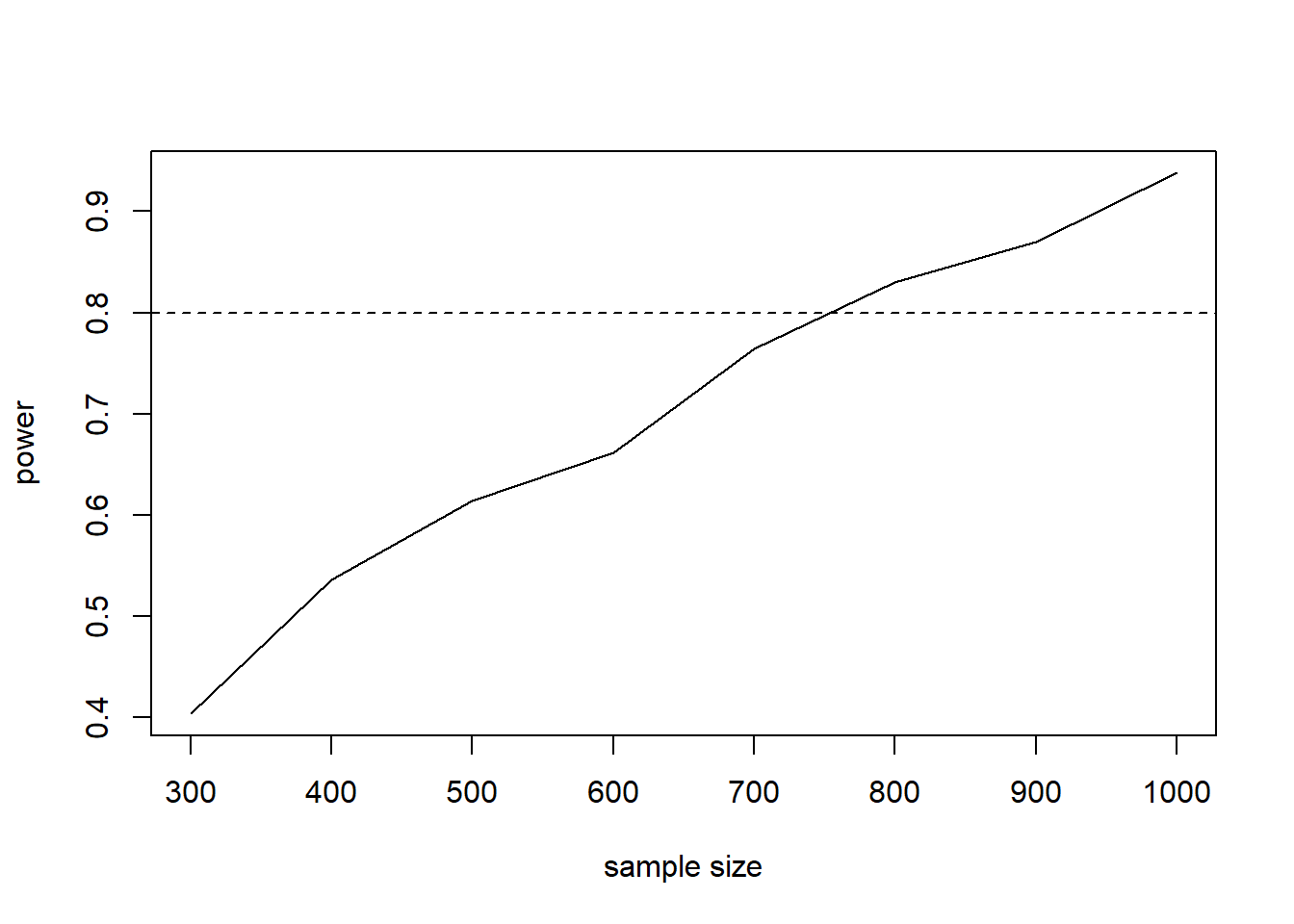
Notice 700 is awfully close to our desired power of 0.8. Perhaps we should try 1000 simulations instead of 500. We’ll leave that to the interested reader.
R session details
Analyses were conducted using the R Statistical language (version 4.5.1; R Core Team, 2025) on Windows 11 x64 (build 26100).
Clay Ford
Statistical Research Consultant
University of Virginia Library
May 4, 2019
Updated May 22, 2023
For questions or clarifications regarding this article, contact statlab@virginia.edu.
View the entire collection of UVA Library StatLab articles, or learn how to cite.