
Pairwise comparison means comparing all pairs of something. If I have three items, A, B and C, that means comparing A to B, A to C, and B to C. Given n items, I can determine the number of possible pairs using the binomial coefficient: $$ \frac{n!}{2!(n - 2)!} = \binom {n}{2}$$ Using the R statistical computing environment, we can use the choose() function to quickly calculate this. For example, how many possible 2-item combinations can I "choose" from 10 items?
choose(10,2)
[1] 45
We sometimes want to make pairwise comparisons to see where differences occur. Let's say we go to 8 high schools in an area, survey 30 students at each school, and ask them whether or not they floss their teeth at least once a day. When finished we'll have 8 proportions of students who answered "Yes." An obvious first step would be to conduct a hypothesis test for any differences between these proportions. The null would be no difference between the proportions versus some difference. If we reject the null, we have evidence of differences. But where are the differences? This leads us to pairwise comparisons of proportions, where we make multiple comparisons. The outcome of these pairwise comparisons will hopefully tell us which schools have significantly different proportions of students flossing.
Making multiple comparisons leads to an increased chance of making a false discovery, i.e., rejecting a null hypothesis that should not have been rejected. When we run a hypothesis test, we always run a risk of finding something that isn't there. Think of flipping a fair coin 10 times and getting 9 or 10 heads (or 0 or 1 heads). That's improbable but not impossible. If it happened to us we may conclude the coin is unfair, but that would be the wrong conclusion if the coin truly was fair. It just so happened we were very unlucky to witness such an unusual event. As we said, the chance of this happening is low in a single trial, but we increase the chance of it happening by conducting multiple trials.
The probability of observing 0, 1, 9, or 10 heads when flipping a fair coin 10 times is about 0.02 which can be calculated in R as follows:
pbinom(q = 1, size = 10, prob = 0.5) * 2
[1] 0.02148438
Therefore the the probability of getting 2 - 8 heads is about 0.98:
1 - pbinom(q = 1, size = 10, prob = 0.5) * 2
[1] 0.9785156
The probability of getting 2 - 8 heads in 10 trials is 0.98 multiplied by itself 10 times:
(1 - pbinom(q = 1, size = 10, prob = 0.5) * 2)^10
[1] 0.8047809
Therefore the probability of getting 0, 1, 9, or 10 heads in 10 trials is now about 0.20:
1 - (1 - pbinom(q = 1, size = 10, prob = 0.5) * 2)^10
[1] 0.1952191
We can think of this as doing multiple hypothesis tests. Flip 10 coins 10 times each, get the proportion of heads for each coin, and use 10 one-sample proportion tests to statistically determine if the results we got are consistent with a fair coin. In other words, do we get any p-values less than, say, 0.05?
We can simulate this in R. First we replicate 1,000 times the act of flipping 10 fair coins 10 times each and counting the number of heads using the rbinom() function. This produces a 10 x 1000 matrix of results that we save as coin.flips. We then apply a function to each column of the matrix that runs 10 one-sample proportion tests using the prop.test() function and saves a TRUE/FALSE value if any of the p-values are less than 0.05 (we talk more about the prop.test() function below). This returns a vector we save as results that contains TRUE or FALSE for each replicate. R treats TRUE and FALSE as 0 or 1, so calling mean() on results returns the proportion of TRUE values in the vector. We get about 0.20, confirming our calculations. (If you run the code below you'll probably get a slightly different but similar answer.)
trials <- 10
coin.flips <- replicate(1000, rbinom(n = 10, size = trials, prob = 0.5))

multHypTest <- function(x){
  pvs <- sapply(x, function(x)prop.test(x = x, n = trials, p = 0.5)$p.value)
  any(pvs < 0.05)
}

results <- apply(coin.flips,2,multHypTest)
mean(results)
[1] 0.206
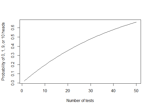
That's just for 10 trials. What about 15 or 20 or more? You can re-run the code above with trials set to a different value. We can also visualize it by plotting the probability of an unusual result (0, 1, 9, or 10 heads) versus the number of trials. Notice how rapidly the probability of a false discovery increases with the number of trials.
curve(expr = 1 - (1 - pbinom(q = 1, size = 10, prob = 0.5) * 2)^x,
      xlim = c(1,50),
      xlab = "Number of tests",
      ylab = "Probability of 0, 1, 9, or 10 heads")
So what does all of this tell us? It reveals that traditional significance levels such as 0.05 are too high when conducting multiple hypothesis tests. We need to either adjust our significance level or adjust our p-values. As we'll see, the usual approach is to adjust the p-values using one of several methods for p-value adjustment.
Let's return to our example of examining the proportion of high school students (sample size 30 at each school) who floss at 8 different high schools. We'll simulate this data as if the true proportion is 30% at each school (i.e., no difference). We use set.seed() to make the data reproducible.
set.seed(15)
n <- 30
k <- 8
school <- rep(1:k, each = n)
floss <- replicate(k, sample(x = c("Y","N"),
                             size = n,
                             prob = c(0.3, 0.7),
                             replace = TRUE))
dat <- data.frame(school, floss = as.vector(floss))
With our data generated, we can tabulate the number of Yes and No responses at each school:
flossTab <- with(dat, table(school, floss))
flossTab
      floss
school  N  Y
     1 18 12
     2 19 11
     3 14 16
     4 19 11
     5 26  4
     6 15 15
     7 20 10
     8 21  9
Using prop.table() we can determine the proportions. Specifying margin = 1 means proportions are calculated across the rows for each school. (We also round to two decimal places for presentation purposes.) The second column contains the proportion of students who answered Yes at each school.
round(prop.table(flossTab, margin = 1),2)
      floss
school    N    Y
     1 0.60 0.40
     2 0.63 0.37
     3 0.47 0.53
     4 0.63 0.37
     5 0.87 0.13
     6 0.50 0.50
     7 0.67 0.33
     8 0.70 0.30
First we might want to run a test to see if we can statistically conclude that not all proportions are equal. We can do this with the prop.test() function. The prop.test() function requires that Yes (or "success") counts be in the first column of a table and No (or "failure") counts in the second column. Thus we switch the columns using subsetting brackets with a vector indicating column order.
prop.test(flossTab[,c("Y","N")])
	8-sample test for equality of proportions without continuity correction

data:  flossTab[, c("Y", "N")]
X-squared = 13.78, df = 7, p-value = 0.05524
alternative hypothesis: two.sided
sample estimates:
   prop 1    prop 2    prop 3    prop 4    prop 5    prop 6    prop 7    prop 8
0.4000000 0.3666667 0.5333333 0.3666667 0.1333333 0.5000000 0.3333333 0.3000000
The p-value of 0.055 is borderline significant and indicates some evidence of differences among proportions. We generated the data, so we know there actually is no difference! But if these were real data that we had spent considerable resources collecting, we might be led to believe (perhaps even want to believe) some differences indeed exist. That p-value is so close to significance! School #5, in particular, with a proportion of 13% looks far lower than school #3 with 53%. We could conclude this hypothesis test is significant at 0.10 level and proceed to pairwise comparisons.
To do that in R we use the pairwise.prop.test() function which requires a table in the same format as prop.test(), with Yes counts in the first column and No counts in the second column:
pairwise.prop.test(x = flossTab[,c("Y","N")])
	Pairwise comparisons using Pairwise comparison of proportions

data:  flossTab[, c("Y", "N")]

  1     2     3     4     5     6     7
2 1.000 -     -     -     -     -     -
3 1.000 1.000 -     -     -     -     -
4 1.000 1.000 1.000 -     -     -     -
5 1.000 1.000 0.073 1.000 -     -     -
6 1.000 1.000 1.000 1.000 0.149 -     -
7 1.000 1.000 1.000 1.000 1.000 1.000 -
8 1.000 1.000 1.000 1.000 1.000 1.000 1.000

P value adjustment method: holm
This produces a table of 28 p-values since there are 28 possible pairs between 8 items. We interpret the table by using row and column numbers to find the p-value for a particular pair. For example the p-value of 0.073 at the intersection of row 5 and column 3 is the p-value for the two-sample proportion test between school #5 and school #3. It appears to be insignificant at the traditional 5% level. All other p-values are clearly insignificant. In fact, most are 1. This is due to the p-value adjustment that was made. The output tells us the "holm" method was used. We won't get into the details of how this method works, but suffice to say it increases the p-values in an effort to adjust for the many comparisons being made. In this case, it does what it's supposed to: It adjusts the p-values and allows us to make a good case there is no differences between schools, at least not at the 5% level, which would be the correct decision.
We can do pairwise comparisons without adjusted p-values by setting p.adjust.method = "none". Let's do that and see what happens:
# NOTE: This analysis is wrong!
pairwise.prop.test(x = flossTab[,c("Y","N")], p.adjust.method = "none")
	Pairwise comparisons using Pairwise comparison of proportions

data:  flossTab[, c("Y", "N")]

  1      2      3      4      5      6      7
2 1.0000 -      -      -      -      -      -
3 0.4376 0.2993 -      -      -      -      -
4 1.0000 1.0000 0.2993 -      -      -      -
5 0.0410 0.0736 0.0026 0.0736 -      -      -
6 0.6038 0.4345 1.0000 0.4345 0.0055 -      -
7 0.7888 1.0000 0.1927 1.0000 0.1270 0.2949 -
8 0.5883 0.7842 0.1161 0.7842 0.2100 0.1876 1.0000

P value adjustment method: none
Notice now we have significant differences for 3 pairs: (5,1), (5,3), and (6,5). Again we know this is wrong because we simulated the data. The truth is all schools have a floss rate of 30%. But we see that through random chance and not adjusting our p-values for multiple testing we got what look to be significant results. This illustrates the importance of using adjusted p-values when making multiple comparisons.
There are other p-value adjustment methods available. A common and conservative choice is the bonferroni method. It simply multiplies all p-values by the number of pairs. In our example that is 28. To see all p-value adjustment methods available in R, enter ?p.adjust at the console.
R session details
Analyses were conducted using the R Statistical language (version 4.5.2; R Core Team, 2025) on Windows 11 x64 (build 26100).
References
- Holm S (1979). A simple sequentially rejective multiple test procedure. Scandinavian Journal of Statistics, 6, 65–70. https://www.jstor.org/stable/4615733.
- R Core Team (2025). R: A Language and Environment for Statistical Computing. R Foundation for Statistical Computing, Vienna, Austria. https://www.R-project.org/.
Clay Ford
Statistical Research Consultant
University of Virginia Library
October 20, 2016
For questions or clarifications regarding this article, contact statlab@virginia.edu.
View the entire collection of UVA Library StatLab articles, or learn how to cite.