Hierarchical Linear Regression

Note: This post is not about hierarchical linear modeling (HLM; multilevel modeling). Hierarchical regression is model comparison of nested regression models.

When do I want to perform hierarchical regression analysis?

Hierarchical regression is a way to show if variables of interest explain a statistically significant amount of variance in your dependent variable (DV) after accounting for all other variables. This is a framework for model comparison rather than a statistical method. In this framework, you build several regression models by adding variables to a previous model at each step; later models always include smaller models in previous steps. In many cases, our interest is to determine whether newly added variables show a significant improvement in \(R^2\) (the proportion of DV variance explained by the model).

Let’s say we’re interested in the relationship between social interaction and happiness. In this line of research, number of friends has been a known predictor in addition to demographic characteristics. However, we’d like to investigate if the number of pets could be an important predictor for happiness.

The first model (Model 1) typically includes demographic information such as age, gender, ethnicity, and education. In the next step (Model 2), we could add known important variables in this line of research. Here we would replicate previous research in this subject area. In the following step (Model 3), we could add the variables that we’re interested in.

• Model 1: Happiness = Intercept + Age + Gender (\(R^2\) = .029)
• Model 2: Happiness = Intercept + Age + Gender + # of friends (\(R^2\) = .131)
• Model 3: Happiness = Intercept + Age + Gender + # of friends + # of pets (\(R^2\) = .197, \(\Delta R^2\) = .066)

Our interest is whether Model 3 explains the DV better than Model 2. If the difference of \(R^2\) between Model 2 and 3 is statistically significant, we can say the added variables in Model 3 explain the DV above and beyond the variables in Model 2. In this example, we’d like to know if the .066 increase in \(R^2\) (.197 - .131 = .066) is statistically significant. If so, we can say that the number of pets explains an additional 6% of the variance in happiness and it is statistically significant.

There are many different ways to examine research questions using hierarchical regression. We can add multiple variables at each step. We can have only two models or more than three models depending on the research question(s). We can run regressions on multiple different DVs and compare the results for each DV.

Conceptual Steps

Depending on statistical software, we can run hierarchical regression with one click (SPSS) or do it manually step-by-step (R). Regardless, it’s helpful to understand how this works conceptually.

• Build sequential (nested) regression models by adding a variable(s) at each step.
• Run ANOVAs (to compute \(R^2\)) and regressions (to obtain coefficients).
• Compare sums of squares between models from ANOVA results.
  • Compute a difference in sum of squares (\(SS\)) at each step.
  • Find corresponding F-statistics and p-values for the \(SS\) differences.
• Compute increased \(R^2\)s from the \(SS\) differences.
  • \(R^2 = \frac{SS_{Explained}}{SS_{Total}}\)

Examples in R

In R, we can find sums of squares and corresponding F-statistics and p-values using anova(). When we use anova() with a single model, it shows analysis of variance for each variable. However, when we use anova() with multiple models, it does model comparisons. Either way, to use anova(), we need to run linear regressions first.

# Import data (simulated data for this example)
myData <- read.csv('http://static.lib.virginia.edu/statlab/materials/data/hierarchicalRegressionData.csv')

# Build models
m0 <- lm(happiness ~ 1, data=myData)  # to obtain Total SS
m1 <- lm(happiness ~ age + gender, data=myData)  # Model 1
m2 <- lm(happiness ~ age + gender + friends, data=myData)  # Model 2
m3 <- lm(happiness ~ age + gender + friends + pets, data=myData)  # Model 3

After regressions are run (obtaining lm objects), anova() is run with the lm objects. When we regress the DV on an intercept without predictors (m0 in this example), anova() results show Total \(SS\).

anova(m0)  # to obtain Total SS

Analysis of Variance Table

Response: happiness
          Df Sum Sq Mean Sq F value Pr(>F)
Residuals 99 240.84  2.4327  

Total \(SS\) is 240.84. We will use this value to compute \(R^2\)s later. Next, compare \(SS\) of the three models that we have built.

anova(m1, m2, m3)  # model comparison

Analysis of Variance Table

Model 1: happiness ~ age + gender
Model 2: happiness ~ age + gender + friends
Model 3: happiness ~ age + gender + friends + pets
  Res.Df    RSS Df Sum of Sq       F    Pr(>F)    
1     97 233.97                                   
2     96 209.27  1    24.696 12.1293 0.0007521 ***
3     95 193.42  1    15.846  7.7828 0.0063739 ** 
---
Signif. codes:  0 ‘***’ 0.001 ‘**’ 0.01 ‘*’ 0.05 ‘.’ 0.1 ‘ ’ 1

• Model 0: \(SS_{Total}\) = 240.84 (no predictors)
• Model 1: \(SS_{Residual}\) = 233.97 (after adding age and gender)
• Model 2: \(SS_{Residual}\) = 209.27, \(SS_{Difference}\) = 24.696, \(F\)(1,96) = 12.1293, \(p\) = 0.0007521 (after adding friends)
• Model 3: \(SS_{Residual}\) = 193.42, \(SS_{Difference}\) = 15.846, \(F\)(1,95) = 7.7828, \(p\) = 0.0063739 (after adding pets)

By adding friends, the model sum of squares decreased by 24.696, a statistically significant change according to the corresponding F-statistic and p-value. The \(R^2\) increased by .103 (24.6957 / 240.84 = 0.1025399) in Model 2. By adding pets, the model accounts for additional \(SS\) 15.846 and it was statistically significant again. The \(R^2\) increased by .066 (15.8461 / 240.84 = 0.06579513) in Model 3.

summary() of an lm object shows coefficients of variables:

summary(m1)

Coefficients:
            Estimate Std. Error t value Pr(>|t|)    
(Intercept)  7.66778    2.01364   3.808 0.000246 ***
age         -0.13039    0.07936  -1.643 0.103611    
genderMale   0.16430    0.31938   0.514 0.608106    
---
Signif. codes:  0 ‘***’ 0.001 ‘**’ 0.01 ‘*’ 0.05 ‘.’ 0.1 ‘ ’ 1

Residual standard error: 1.553 on 97 degrees of freedom
Multiple R-squared:  0.02855,	Adjusted R-squared:  0.008515 
F-statistic: 1.425 on 2 and 97 DF,  p-value: 0.2455

summary(m2)

Coefficients:
            Estimate Std. Error t value Pr(>|t|)   
(Intercept)  6.21730    1.96220   3.169  0.00206 **
age         -0.12479    0.07546  -1.654  0.10146   
genderMale   0.14931    0.30365   0.492  0.62405   
friends      0.18985    0.05640   3.366  0.00110 **
---
Signif. codes:  0 ‘***’ 0.001 ‘**’ 0.01 ‘*’ 0.05 ‘.’ 0.1 ‘ ’ 1

Residual standard error: 1.476 on 96 degrees of freedom
Multiple R-squared:  0.1311,	Adjusted R-squared:  0.1039 
F-statistic: 4.828 on 3 and 96 DF,  p-value: 0.003573

summary(m3)

Coefficients:
            Estimate Std. Error t value Pr(>|t|)   
(Intercept)  5.78540    1.90266   3.041  0.00305 **
age         -0.11146    0.07309  -1.525  0.13057   
genderMale  -0.14267    0.31157  -0.458  0.64806   
friends      0.17134    0.05491   3.120  0.00239 **
pets         0.36391    0.13044   2.790  0.00637 **
---
Signif. codes:  0 ‘***’ 0.001 ‘**’ 0.01 ‘*’ 0.05 ‘.’ 0.1 ‘ ’ 1

Residual standard error: 1.427 on 95 degrees of freedom
Multiple R-squared:  0.1969,	Adjusted R-squared:  0.1631 
F-statistic: 5.822 on 4 and 95 DF,  p-value: 0.0003105

Aside from the coefficients of variables, let’s take a look at \(R^2\)s of Model 1, 2, and 3, which are 0.02855, 0.1311, and 0.1969 respectively. The \(R^2\) changes computed using anova() results correspond to differences in \(R^2\)s in lm() results for each model: 0.1311 - 0.02855 = 0.10255 for Model 2 and 0.1969 - 0.1311 = 0.0658 for Model 3 (with rounding errors). Although we can compute \(R^2\) differences between models using lm() results, lm() results don’t provide corresponding F-statistics and p-values to an increased \(R^2\). And it’s important to remember that adding variables always increases \(R^2\), whether or not it actually explains additional variation in the DV. That’s why it’s crucial to perform F-tests and not just rely on the difference in \(R^2\) between models.

What to report as the results?

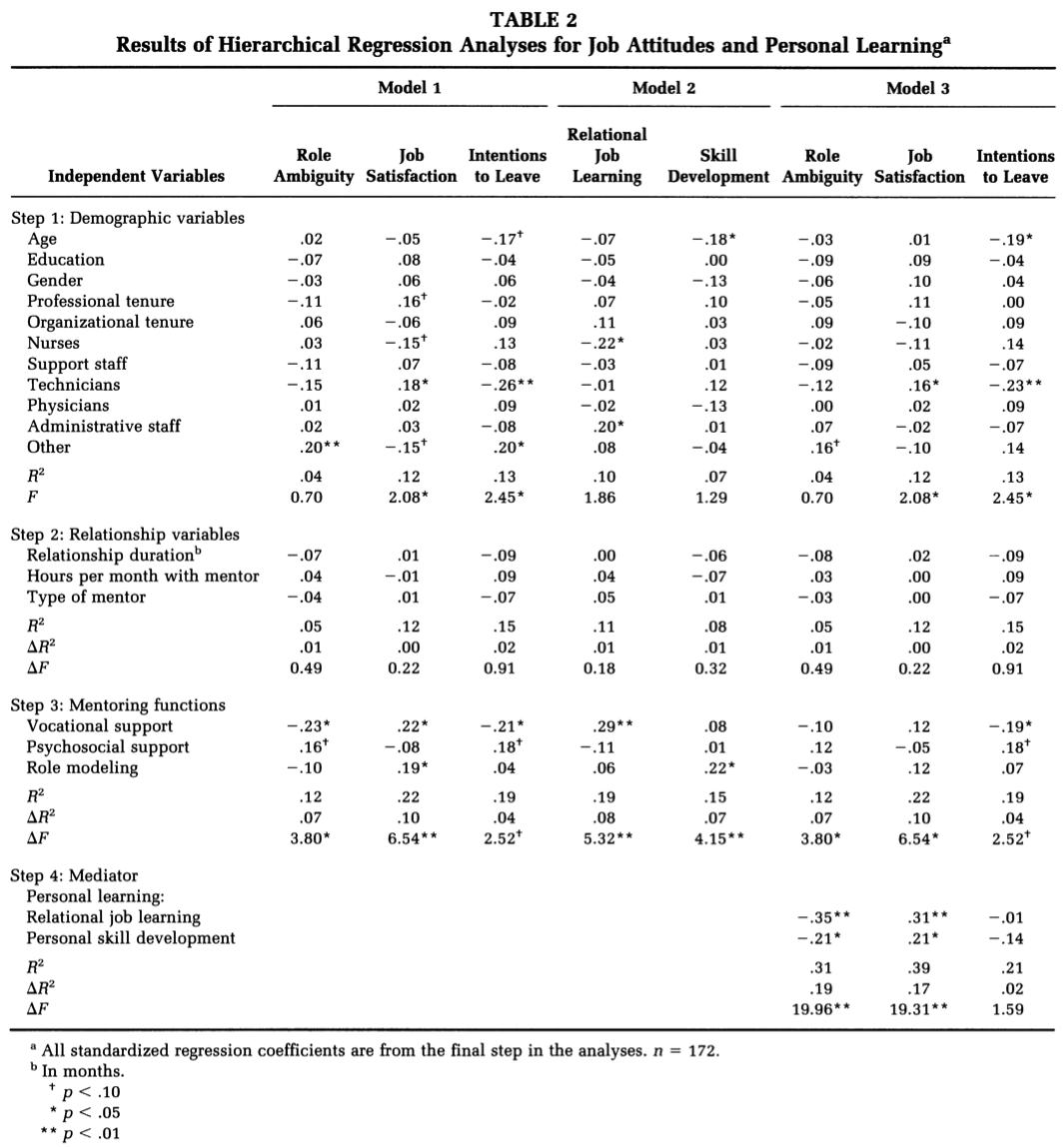
It is common to report coefficients of all variables in each model and differences in \(R^2\) between models. In research articles, the results are typically presented in tables as below. Note that the second example (Lankau & Scandura, 2002) had multiple DVs and ran hierarchical regressions for each DV.

Bommae Kim
Statistical Consulting Associate
University of Virginia Library
May 20, 2016