
A Simple Slopes Analysis is a follow-up procedure to regression modeling that helps us investigate and interpret “significant” interactions. The analysis is often employed for interactions between two numeric predictors, but it can be applied to other types of interactions as well. To motivate why we might be interested in this type of analysis, consider the following research question:
Does the length of time in a managerial position (X) and a manager’s ability (Z) help explain or predict a manager’s self-assurance (Y)?
We might hypothesize that the effect of a manager’s ability (Z) on self-assurance (Y) depends on their tenure at the job (X), and vice versa. In other words, we think these predictors interact. Therefore, when analyzing the data with a regression model, we would model self-assurance (Y) as a function of time at job (X), ability (Z), and their interaction (XZ).
Now this is a hypothetical research question that comes from Aiken and West (1991). In their book they coined the phrase “Simple Slope” analysis and used the above fictitious scenario to present the details. They simulated their data but did not share it. However they described how they simulated data and showed their estimated model, so we were able to simulate our own data and roughly recreate their results. See this GitHub Gist for the simulation details.
Let’s load the fictitious data set and model self-assurance (Y) as a function of length of time (X) and ability (Z), along with their interaction. Below we use R and its workhorse linear modeling function, lm(). We specify we want to model an interaction between X and Z using the formula syntax X + Z + X:Z.
d <- readRDS(url("http://static.lib.virginia.edu/statlab/materials/data/simple.rds"))
m <- lm(Y ~ X + Z + X:Z, data = d)
summary(m)
  Call:
  lm(formula = Y ~ X + Z + X:Z, data = d)

  Residuals:
       Min       1Q   Median       3Q      Max
  -15.9035  -3.5942   0.1004   3.6776  15.4320

  Coefficients:
              Estimate Std. Error t value Pr(>|t|)
  (Intercept)  87.7424     6.3737   13.77   <2e-16 ***
  X           -24.6157     1.2734  -19.33   <2e-16 ***
  Z            -8.7837     0.6083  -14.44   <2e-16 ***
  X:Z           2.5603     0.1179   21.71   <2e-16 ***
  ---
  Signif. codes:  0 '***' 0.001 '**' 0.01 '*' 0.05 '.' 0.1 ' ' 1

  Residual standard error: 5.212 on 396 degrees of freedom
  Multiple R-squared:  0.8276, Adjusted R-squared:  0.8263
  F-statistic: 633.6 on 3 and 396 DF,  p-value: < 2.2e-16
In the summary output, we see the interaction coefficient (X:Z) is estimated as 2.6 with a standard error of about 0.12. It appears we can be confident that this interaction is positive and greater than 2. But what does 2.6 mean? How do the predictors interact exactly?
A common approach to investigating interactions is via effect displays, such as those provided by the effects or ggeffects packages. For example, here’s the ggeffects version created with the ggpredict() function and its associated plot() method. The syntax X[4:6 by=0.5] restricts the range of the x-axis from 4 to 6 in increments of 0.5. This approximates Figure 2.1(b) in Aiken and West (1991).
library(ggeffects)
ggpredict(m, terms = c("X[4:6 by=0.5]", "Z")) |> plot()
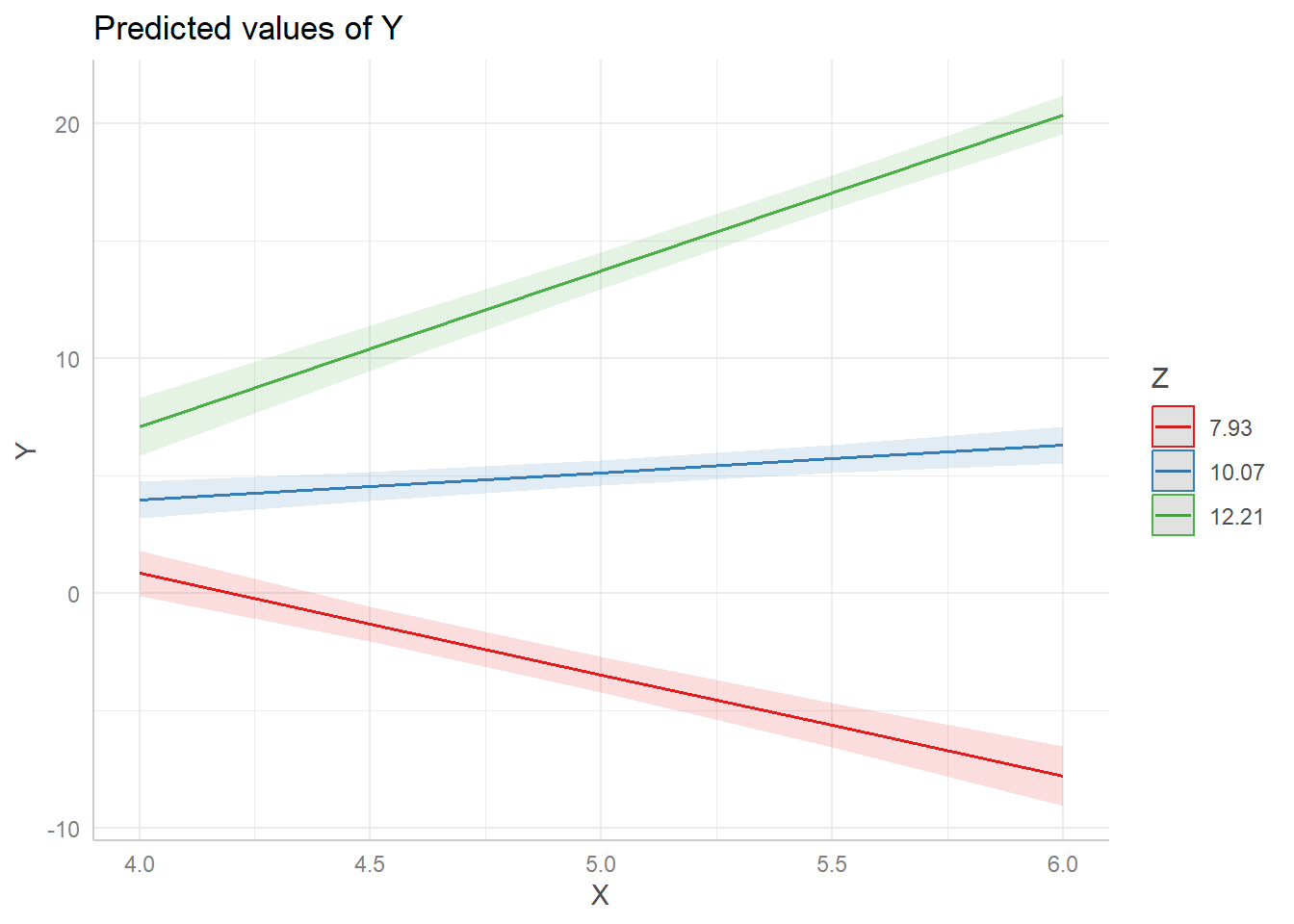
This visualizes our model by showing the relationship between X and Y while Z is held at 3 separate values. By default, the values of Z are set to its mean (10.07), one standard deviation below its mean (7.93), and one standard deviation above its mean (12.21).
When Z is 7.93, the relationship between X and Y is negative (red line). But when Z is 12.21, the relationship between X and Y reverses and becomes positive (green line). This type of plot helps us better understand the nature of the interaction between the two predictors. This would be difficult to infer from just looking at the interaction coefficient in the model output.
The plot is created by using our model to make three sets of predictions:
- Predict Y using a range of X values holding Z at 7.93
- Predict Y using a range of X values holding Z at 10.07
- Predict Y using a range of X values holding Z at 12.21
We can do this “by hand” using the base R predict() function. For example, here are predictions made for X values ranging from 4 through 6 in steps of 0.5 while holding Z at 7.93.
predict(m, newdata = data.frame(X = seq(4, 6, 0.5), Z = 7.93))
           1          2          3          4          5
   0.8389098 -1.3171921 -3.4732941 -5.6293960 -7.7854979
The ggpredict() function does all this for us. By setting terms = c("X[4:6 by=0.1]", "Z"), with the variables in that order, we tell ggpredict() to use the specified range of values for X and to hold Z at fixed values. Calling ggpredict() without plot() shows the predicted values and associated confidence intervals at each prediction. The confidence intervals form the ribbons around the fitted lines in the plot above and help us assess the uncertainty in our predictions.
ggpredict(m, terms = c("X[4:6 by=0.5]", "Z"))
  # Predicted values of Y

  # Z = 7.93

     X | Predicted |         95% CI
  ---------------------------------
  4.00 |      0.84 | [-0.11,  1.79]
  4.50 |     -1.32 | [-2.07, -0.56]
  5.00 |     -3.47 | [-4.23, -2.72]
  5.50 |     -5.63 | [-6.58, -4.68]
  6.00 |     -7.79 | [-9.04, -6.53]

  # Z = 10.07

     X | Predicted |       95% CI
  -------------------------------
  4.00 |      3.96 | [3.17, 4.75]
  4.50 |      4.54 | [3.93, 5.16]
  5.00 |      5.13 | [4.59, 5.66]
  5.50 |      5.71 | [5.11, 6.31]
  6.00 |      6.29 | [5.52, 7.06]

  # Z = 12.21

     X | Predicted |         95% CI
  ---------------------------------
  4.00 |      7.08 | [ 5.87,  8.29]
  4.50 |     10.40 | [ 9.44, 11.36]
  5.00 |     13.72 | [12.94, 14.51]
  5.50 |     17.05 | [16.32, 17.77]
  6.00 |     20.37 | [19.55, 21.19]
The objective of a Simple Slopes analysis is to quantify the slopes in effect displays. For example, in the plot above, the green line shows us that the relationship between Y (self-assurance) and X (length of time) is positive when Z (ability) is 12.21. But what is the slope of that line?
One way to carry out a Simple Slopes analysis in R is to use the emtrends() function from the emmeans package. Below we first calculate the Z values at which we want to estimate the simple slopes and save as a vector called “zvals”. These are the same values of Z that ggpredict() used. Then we use the emtrends() function on our model object, m, with specs = "Z, var = "X" to specify that we want to estimate the slopes of X at specific values of Z. We use the at argument to indicate which Z values we want to use, which needs to be entered as a named list.
library(emmeans)
zvals <- c(mean(d$Z) - sd(d$Z), mean(d$Z), mean(d$Z) + sd(d$Z))
emtrends(m, specs = "Z", var = "X", at = list(Z = zvals))
       Z X.trend    SE  df lower.CL upper.CL
    7.93   -4.31 0.416 396   -5.128    -3.49
   10.07    1.17 0.287 396    0.606     1.73
   12.21    6.65 0.344 396    5.972     7.33

  Confidence level used: 0.95
The output tells us in the first row under the “X.trend” column that the slope of the red line in our effect display is about -4.31, with a 95% confidence interval of [-5.13, -3.49]. This tells us that when a manager’s ability (Z) is one standard deviation below the mean (-4.31), we can expect each additional year in the managerial position (X) to decrease self-assurance (Y) by about 4 points on average. In the last row we see that when a manager’s ability (Z) is one standard deviation above the mean (12.21), we can expect each additional year in the managerial position (X) to increase self-assurance (Y) by about 6 points on average.
Although the confidence intervals make it clear these slopes are “significantly” different from 0, some researchers still need to report hypothesis tests and p-values. To obtain such results, we can pipe the output of emtrends() into the test() function.
emtrends(m, specs = "Z", var = "X", at = list(Z = zvals)) |> test()
       Z X.trend    SE  df t.ratio p.value
    7.93   -4.31 0.416 396 -10.356  <.0001
   10.07    1.17 0.287 396   4.082  0.0001
   12.21    6.65 0.344 396  19.318  <.0001
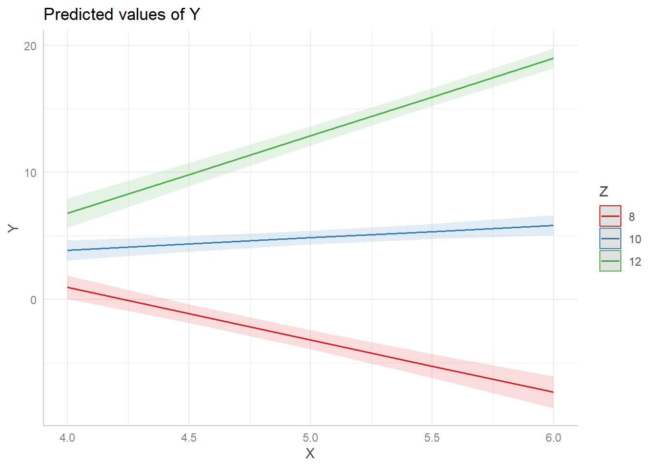
Traditionally, one of the interacting predictors is held at their mean, one standard deviation above the mean, and one standard deviation below the mean. That’s the default in the ggpredict() function, what Aiken and West presented in their seminal example, and what we did above. However, there is no reason this cannot be changed to other values that are more reasonable for the research question at hand. There may be specific values of interest, or it may be more reasonable to use the 25th, 50th, and 75th percentiles, particularly if the data are skewed. You’re also not limited to 3 values, though 3 values often captures the gist of interactions between numeric values quite well.
Returning to our example, let’s use the “pretty” values of 8, 10 and 12. Perhaps Z (manager ability) is measured in whole numbers. First we redo the plot. Notice we use the syntax Z[8,10,12] to specify we want to fix Z at 8, 10, and 12. (This syntax is specific to the ggeffects package.)
ggpredict(m, terms = c("X[4:6 by=0.5]", "Z[8,10,12]")) |> plot()
And now we use emtrends() to carry our the Simple Slopes analysis using our updated Z values.
zvals <- c(8,10,12)
emtrends(m, specs = "Z", var = "X", at = list(Z = zvals))
    Z X.trend    SE  df lower.CL upper.CL
    8  -4.133 0.410 396   -4.939    -3.33
   10   0.988 0.288 396    0.421     1.55
   12   6.108 0.330 396    5.459     6.76

  Confidence level used: 0.95
The estimated slopes change slightly, but the substance of the results is the same. Again, the fixed values you choose should be values of interest. You should not reflexively rely on the mean and +/- 1 SD. It’s also worth considering if the fixed values are plausible for the entire range of predictor values being used to create the slope. For example, is it plausible that someone with very low ability (Z) as a manager would stay in the job for 5 or 6 years (X)? (A cynical workforce veteran might say that’s not only plausible but probable!) A good indicator that you’re entertaining implausible interactions will be wide and uncertain confidence ribbons around portions of the slopes in your effect display. This means your model is trying to make predictions using sparse or unavailable data.
The biggest consideration of all is whether or not your model is any good. A significant interaction doesn’t necessarily mean your model is doing a good job of explaining variability in your response. All the usual model checks and diagnostics that accompany regression modeling should be carried out before proceeding to a Simple Slopes analysis.
We now present some technical details for the interested reader.
Quantifying slopes
The slopes are determined by plugging in our fixed predictor values and simplifying the model. In our example above, the fitted model is (with coefficients rounded to one decimal place)
\[Y = 87.7 + -24.6X + -8.8Z + 2.6XZ\]
The simple slope when Z = 12 is
\[Y = 87.7 + -24.6X + -8.8(12) + 2.6X(12) \]
\[Y = [87.7 + -8.8(12)] + [-24.6X + 2.6X(12)]\]
\[Y = -17.7 + 6.1X\]
Which matches the slope reported by emmeans above. Similar calculations can be carried out by plugging in Z = 10 and Z = 8.
Standard errors for slopes
Standard errors quantify uncertainty in estimates. Our estimated slope above is 6.1, but it’s just an estimate. A different sample would produce a different estimate. The standard error provides some indication of how much this estimate might change from sample to sample.
The estimated slope is a combination of two estimated parameters, -24.6 and 2.6:
\[-24.6X + 2.6X(12)\]
These parameters have estimated variances in the 2nd and 4th positions on the diagonal of the model variance-covariance matrix, which can be viewed with the vcov() function.
vcov(m)
              (Intercept)          X           Z         X:Z
  (Intercept)   40.623919 -7.9397209 -3.77396659  0.72801998
  X             -7.939721  1.6216245  0.72525452 -0.14647100
  Z             -3.773967  0.7252545  0.37007794 -0.07008505
  X:Z            0.728020 -0.1464710 -0.07008505  0.01390898
The square root of the diagonal values are the standard errors reported in the model output. (Compare to model summary above.)
vcov(m) |> diag() |> sqrt()
  (Intercept)           X           Z         X:Z
    6.3736896   1.2734302   0.6083403   0.1179363
It turns out the standard error of combinations of parameters can be estimated with the following formula:
\[\sigma_{\text{comb}}^2 = w'\Sigma_bw \]
Where w represents weights of the combination and \(\Sigma_b\) is the variance-covariance function of the parameters. The weights in our combination above are 0, 1, 0, and 12. The weights on the first and third parameters are 0 because our linear combination does not involve them. The weights on the second and fourth parameters are 1 and 12, because the second is added to the fourth after it’s multiplied by 12. We can carry out this calculation using matrix algebra as follows. We take the square root of the result to convert variance to standard error. Notice the result matches the standard error reported by emmeans for Z = 12.
sqrt(t(c(0,1,0,12)) %*% vcov(m) %*% c(0,1,0,12))
            [,1]
  [1,] 0.3304753
The standard error is small relative to the estimated slope and gives us confidence that the true slope is reliably positive and close to 6.
An algebraic expression of the standard error calculation is
\[\sigma_{\text{comb}}^2 = s_{22} + 2Zs_{24}+ Z^2s_{44} \]
Where the s refers to the model variance-covariance matrix and the subscripts refer to locations in the matrix. Notice the middle term includes the covariance between the 2nd and 4th parameters. Again we take the square root to get standard error.
\[0.3304753 = \sqrt{1.6216245 + 2(12)(-0.14647100) + 12^2(0.01390898)} \]
Or using R:
s <- vcov(m)
sqrt(s[2,2] + 2*12*s[2,4] + 12^2*(s[4,4]))
[1] 0.3304753
Confidence intervals and test statistics
The confidence interval is computed by adding and subtracting the standard error, multiplied by the 95th quantile of a t distribution with model degrees of freedom, to the estimated slope. The qt() function provides a quantile for a stated probability and degrees of freedom. For a 95% confidence interval, we either use 0.025 or 0.975. Since we had 400 observations and estimated 4 model parameters, we have 396 degrees of freedom. For Z = 12, our confidence interval is calculated as follows.
6.108 + c(-1,1)*0.330*qt(0.975, df = 396)
[1] 5.459229 6.756771
The test statistic is the estimated slope divided by the standard error. The p-value for a 2-sided null hypothesis test can be calculated using the pt() function. The result in this case is a p-value that is practically 0.
t.stat <- 6.108/0.330
t.stat
[1] 18.50909
pt(q = t.stat, df = 396, lower.tail = F) * 2
[1] 1.474227e-55
R session details
The analysis was done using the R Statistical language (v4.5.1; R Core Team, 2025) on Windows 11 x64, using the packages emmeans (v1.11.2) and ggeffects (v2.3.0).
References
- Aiken, L. S. and West, S.G. (1991). Multiple Regression: Testing and Interpreting Interactions. Newbury Park, Calif: Sage Publications.
- Lenth, R. (2023). emmeans: Estimated Marginal Means, aka Least-Squares Means. https://CRAN.R-project.org/package=emmeans.
- Lüdecke, D. (2018). “ggeffects: Tidy Data Frames of Marginal Effects from Regression Models.” Journal of Open Source Software, 3(26), 772. doi:10.21105/joss.00772 https://doi.org/10.21105/joss.00772.
- R Core Team (2022). R: A language and environment for statistical computing. R Foundation for Statistical Computing, Vienna, Austria. URL https://www.R-project.org/.
Clay Ford
Statistical Research Consultant
University of Virginia Library
March 17, 2023
For questions or clarifications regarding this article, contact statlab@virginia.edu.
View the entire collection of UVA Library StatLab articles, or learn how to cite.