
Multivariate Multiple Regression is a method of modeling multiple responses, or dependent variables, with a single set of predictor variables. For example, we might want to model both math and reading SAT scores as a function of gender, race, parent income, and so forth. This allows us to evaluate the relationship of, say, gender with each score. You may be thinking, "why not just run separate regressions for each dependent variable?" That's actually a good idea! And in fact that's pretty much what multivariate multiple regression does. It regresses each dependent variable separately on the predictors. However, because we have multiple responses, we have to modify our hypothesis tests for regression parameters and our confidence intervals for predictions.
To get started, let's read in some data from the book Applied Multivariate Statistical Analysis (6th ed.) by Richard Johnson and Dean Wichern. This data come from exercise 7.25 and involve 17 overdoses of the drug amitriptyline (Rudorfer, 1982). There are two responses we want to model: TOT and AMI. TOT is total TCAD plasma level and AMI is the amount of amitriptyline present in the TCAD plasma level. The predictors are as follows:
- GEN, gender (male = 0, female = 1)
- AMT, amount of drug taken at time of overdose
- PR, PR wave measurement
- DIAP, diastolic blood pressure
- QRS, QRS wave measurement
We'll use the R statistical computing environment to demonstrate multivariate multiple regression. The following code reads the data into R and names the columns.
ami_data <- read.table("http://static.lib.virginia.edu/statlab/materials/data/ami_data.DAT")
names(ami_data) <- c("TOT","AMI","GEN","AMT","PR","DIAP","QRS")
Before going further you may wish to explore the data using the summary() and pairs() functions.
summary(ami_data)
pairs(ami_data)
Performing multivariate multiple regression in R requires wrapping the multiple responses in the cbind() function. cbind() takes two vectors, or columns, and "binds" them together into two columns of data. We insert that on the left side of the formula operator: ~. On the other side we add our predictors. The + signs do not mean addition but rather inclusion. Taken together the formula cbind(TOT, AMI) ~ GEN + AMT + PR + DIAP + QRS translates to "model TOT and AMI as a function of GEN, AMT, PR, DIAP and QRS." To fit this model we use the workhorse lm() function and save it to an object we name "mlm1". Finally we view the results with summary().
mlm1 <- lm(cbind(TOT, AMI) ~ GEN + AMT + PR + DIAP + QRS, data = ami_data)
summary(mlm1)
Response TOT :

Call:
lm(formula = TOT ~ GEN + AMT + PR + DIAP + QRS, data = ami_data)

Residuals:
   Min     1Q Median     3Q    Max
-399.2 -180.1    4.5  164.1  366.8

Coefficients:
              Estimate Std. Error t value Pr(>|t|)
(Intercept) -2.879e+03  8.933e+02  -3.224 0.008108 **
GEN          6.757e+02  1.621e+02   4.169 0.001565 **
AMT          2.848e-01  6.091e-02   4.677 0.000675 ***
PR           1.027e+01  4.255e+00   2.414 0.034358 *
DIAP         7.251e+00  3.225e+00   2.248 0.046026 *
QRS          7.598e+00  3.849e+00   1.974 0.074006 .
---
Signif. codes:  0 ‘***’ 0.001 ‘**’ 0.01 ‘*’ 0.05 ‘.’ 0.1 ‘ ’ 1

Residual standard error: 281.2 on 11 degrees of freedom
Multiple R-squared:  0.8871,	Adjusted R-squared:  0.8358
F-statistic: 17.29 on 5 and 11 DF,  p-value: 6.983e-05


Response AMI :

Call:
lm(formula = AMI ~ GEN + AMT + PR + DIAP + QRS, data = ami_data)

Residuals:
    Min      1Q  Median      3Q     Max
-373.85 -247.29  -83.74  217.13  462.72

Coefficients:
              Estimate Std. Error t value Pr(>|t|)
(Intercept) -2.729e+03  9.288e+02  -2.938 0.013502 *
GEN          7.630e+02  1.685e+02   4.528 0.000861 ***
AMT          3.064e-01  6.334e-02   4.837 0.000521 ***
PR           8.896e+00  4.424e+00   2.011 0.069515 .
DIAP         7.206e+00  3.354e+00   2.149 0.054782 .
QRS          4.987e+00  4.002e+00   1.246 0.238622
---
Signif. codes:  0 ‘***’ 0.001 ‘**’ 0.01 ‘*’ 0.05 ‘.’ 0.1 ‘ ’ 1

Residual standard error: 292.4 on 11 degrees of freedom
Multiple R-squared:  0.8764,	Adjusted R-squared:  0.8202
F-statistic:  15.6 on 5 and 11 DF,  p-value: 0.0001132
Notice the summary shows the results of two regressions: one for TOT and one for AMI. These are exactly the same results we would get if we modeled each separately. You can verify this for yourself by running the following code and comparing the summaries to what we got above. They're identical.
m1 <- lm(TOT ~ GEN + AMT + PR + DIAP + QRS, data = ami_data)
summary(m1)
m2 <- lm(AMI ~ GEN + AMT + PR + DIAP + QRS, data = ami_data)
summary(m2)
The same diagnostics we check for models with one predictor should be checked for these as well. For a review of some basic but essential diagnostics see our post Understanding Diagnostic Plots for Linear Regression Analysis.
We can use R's extractor functions with our mlm1 object, except we'll get double the output. For example, instead of one set of residuals, we get two:
head(resid(mlm1))
         TOT        AMI
1  132.82172  161.52769
2  -72.00392 -264.35329
3 -399.24769 -373.85244
4 -382.84730 -247.29456
5 -152.39129   15.78777
6  366.78644  217.13206
Instead of one set of fitted values, we get two:
head(fitted(mlm1))
        TOT       AMI
1 3256.1783 2987.4723
2 1173.0039  917.3533
3 1530.2477 1183.8524
4  978.8473  695.2946
5 1048.3913  828.2122
6 1400.2136 1232.8679
Instead of one set of coefficients, we get two:
coef(mlm1)
                      TOT           AMI
(Intercept) -2879.4782461 -2728.7085444
GEN           675.6507805   763.0297617
AMT             0.2848511     0.3063734
PR             10.2721328     8.8961977
DIAP            7.2511714     7.2055597
QRS             7.5982397     4.9870508
Instead of one residual standard error, we get two:
sigma(mlm1)
     TOT      AMI
281.2324 292.4363
Again these are all identical to what we get by running separate models for each response. The similarity ends, however, with the variance-covariance matrix of the model coefficients. We don't reproduce the output here because of the size, but we encourage you to view it for yourself:
vcov(mlm1)
The main takeaway is that the coefficients from both models covary. That covariance needs to be taken into account when determining if a predictor is jointly contributing to both models. For example, the effects of PR and DIAP seem borderline. They appear significant for TOT but less so for AMI. But it's not enough to eyeball the results from the two separate regressions. We should formally test for their inclusion. And that test involves the covariances between the coefficients in both models.
Determining whether or not to include predictors in a multivariate multiple regression requires the use of multivariate test statistics. These are often taught in the context of MANOVA, or multivariate analysis of variance. Again the term "multivariate" here refers to multiple responses or dependent variables. This means we use modified hypothesis tests to determine whether a predictor contributes to a model.
The easiest way to do this is to use the Anova() or Manova() functions in the car package (Fox and Weisberg, 2011), like so:
library(car)
Anova(mlm1)
Type II MANOVA Tests: Pillai test statistic
     Df test stat approx F num Df den Df   Pr(>F)
GEN   1   0.65521   9.5015      2     10 0.004873 **
AMT   1   0.69097  11.1795      2     10 0.002819 **
PR    1   0.34649   2.6509      2     10 0.119200
DIAP  1   0.32381   2.3944      2     10 0.141361
QRS   1   0.29184   2.0606      2     10 0.178092
---
Signif. codes:  0 ‘***’ 0.001 ‘**’ 0.01 ‘*’ 0.05 ‘.’ 0.1 ‘ ’ 1
The results are titled "Type II MANOVA Tests". The Anova() function automatically detects that mlm1 is a multivariate multiple regression object. "Type II" refers to the type of sum-of-squares. This basically says that predictors are tested assuming all other predictors are already in the model. This is usually what we want. Notice that PR and DIAP appear to be jointly insignificant for the two models despite what we were led to believe by examining each model separately.
Based on these results we may want to see if a model with just GEN and AMT fits as well as a model with all five predictors. One way we can do this is to fit a smaller model and then compare the smaller model to the larger model using the anova() function, (notice the little "a"; this is different from the Anova() function in the car package). For example, below we create a new model using the update() function that only includes GEN and AMT. The expression . ~ . - PR - DIAP - QRS says "keep the same responses and predictors except PR, DIAP and QRS."
mlm2 <- update(mlm1, . ~ . - PR - DIAP - QRS)
anova(mlm1, mlm2)
Analysis of Variance Table

Model 1: cbind(TOT, AMI) ~ GEN + AMT + PR + DIAP + QRS
Model 2: cbind(TOT, AMI) ~ GEN + AMT
  Res.Df Df Gen.var.  Pillai approx F num Df den Df Pr(>F)
1     11       43803
2     14  3    51856 0.60386   1.5859      6     22 0.1983
The large p-value provides good evidence that the model with two predictors fits as well as the model with five predictors. Notice the test statistic is "Pillai", which is one of the four common multivariate test statistics.
The car package provides another way to conduct the same test using the linearHypothesis() function. The beauty of this function is that it allows us to run the test without fitting a separate model. It also returns all four multivariate test statistics. The first argument to the function is our model. The second argument is our null hypothesis. The linearHypothesis() function conveniently allows us to enter this hypothesis as character phrases. The null entered below is that the coefficients for PR, DIAP and QRS are all 0.
lh.out <- linearHypothesis(mlm1, hypothesis.matrix = c("PR = 0", "DIAP = 0", "QRS = 0"))
lh.out
Sum of squares and products for the hypothesis:
         TOT      AMI
TOT 930348.1 780517.7
AMI 780517.7 679948.4

Sum of squares and products for error:
         TOT      AMI
TOT 870008.3 765676.5
AMI 765676.5 940708.9

Multivariate Tests:
                 Df test stat approx F num Df den Df  Pr(>F)
Pillai            3 0.6038599 1.585910      6     22 0.19830
Wilks             3 0.4405021 1.688991      6     20 0.17553
Hotelling-Lawley  3 1.1694286 1.754143      6     18 0.16574
Roy               3 1.0758181 3.944666      3     11 0.03906 *
---
Signif. codes:  0 ‘***’ 0.001 ‘**’ 0.01 ‘*’ 0.05 ‘.’ 0.1 ‘ ’ 1
The Pillai result is the same as we got using the anova() function above. The Wilks, Hotelling-Lawley, and Roy results are different versions of the same test. The consensus is that the coefficients for PR, DIAP and QRS do not seem to be statistically different from 0. There is some discrepancy in the test results. The Roy test in particular is significant, but this is likely due to the small sample size (n = 17).
Also included in the output are two sum of squares and products matrices, one for the hypothesis and the other for the error. These matrices are used to calculate the four test statistics. These matrices are stored in the lh.out object as SSPH (hypothesis) and SSPE (error). We can use these to manually calculate the test statistics. For example, let SSPH = H and SSPE = E. The formula for the Wilks test statistic is $$ \frac{\begin{vmatrix}\bf{E}\end{vmatrix}}{\begin{vmatrix}\bf{E} + \bf{H}\end{vmatrix}} $$
In R we can calculate that as follows:
E <- lh.out$SSPE
H <- lh.out$SSPH
det(E)/det(E + H)
[1] 0.4405021
Likewise the formula for Pillai is $$ tr[\bf{H}(\bf{H} + \bf{E})^{-1}] $$ tr means trace. That's the sum of the diagonal elements of a matrix. In R we can calculate as follows:
sum(diag(H %*% solve(E + H)))
[1] 0.6038599
The formula for Hotelling-Lawley is $$ tr[\bf{H}\bf{E}^{-1}] $$ In R:
sum(diag(H %*% solve(E)))
[1] 1.169429
And finally the Roy statistics is the largest eigenvalue of \(\bf{H}\bf{E}^{-1}\). In R code:
e.out <- eigen(H %*% solve(E))
max(e.out$values)
[1] 1.075818
Given these test results, we may decide to drop PR, DIAP and QRS from our model. In fact this is model mlm2 that we fit above. Here is the summary:
summary(mlm2)
Response TOT :

Call:
lm(formula = TOT ~ GEN + AMT, data = ami_data)

Residuals:
    Min      1Q  Median      3Q     Max
-756.05 -190.68  -59.83  203.32  560.84

Coefficients:
             Estimate Std. Error t value Pr(>|t|)
(Intercept)  56.72005  206.70337   0.274   0.7878
GEN         507.07308  193.79082   2.617   0.0203 *
AMT           0.32896    0.04978   6.609 1.17e-05 ***
---
Signif. codes:  0 ‘***’ 0.001 ‘**’ 0.01 ‘*’ 0.05 ‘.’ 0.1 ‘ ’ 1

Residual standard error: 358.6 on 14 degrees of freedom
Multiple R-squared:  0.7664,	Adjusted R-squared:  0.733
F-statistic: 22.96 on 2 and 14 DF,  p-value: 3.8e-05


Response AMI :

Call:
lm(formula = AMI ~ GEN + AMT, data = ami_data)

Residuals:
    Min      1Q  Median      3Q     Max
-716.80 -135.83  -23.16  182.27  695.97

Coefficients:
              Estimate Std. Error t value Pr(>|t|)
(Intercept) -241.34791  196.11640  -1.231  0.23874
GEN          606.30967  183.86521   3.298  0.00529 **
AMT            0.32425    0.04723   6.866 7.73e-06 ***
---
Signif. codes:  0 ‘***’ 0.001 ‘**’ 0.01 ‘*’ 0.05 ‘.’ 0.1 ‘ ’ 1

Residual standard error: 340.2 on 14 degrees of freedom
Multiple R-squared:  0.787,	Adjusted R-squared:  0.7566
F-statistic: 25.87 on 2 and 14 DF,  p-value: 1.986e-05
Now let's say we wanted to use this model to estimate mean TOT and AMI values for GEN = 1 (female) and AMT = 1200. We can use the predict() function for this. First we need put our new data into a data frame with column names that match our original data.
nd <- data.frame(GEN = 1, AMT = 1200)
p <- predict(mlm2, nd)
p
       TOT      AMI
1 958.5473 754.0677
This predicts two values, one for each response. Now this is just a prediction and has uncertainty. We usually quantify uncertainty with confidence intervals to give us some idea of a lower and upper bound on our estimate. But in this case we have two predictions from a multivariate model with two sets of coefficients that covary! This means calculating a confidence interval is more difficult. In fact we don't calculate an interval but rather an ellipse to capture the uncertainty in two dimensions.
Unfortunately at the time of this writing there doesn't appear to be a function in R for creating uncertainty ellipses for multivariate multiple regression models with two responses. However, we have written one below you can use called confidenceEllipse(). The details of the function go beyond a "getting started" blog post but it should be easy enough to use. Simply submit the code in the console to create the function. Then use the function with any multivariate multiple regression model object that has two responses. The newdata argument works the same as the newdata argument for predict. Use the level argument to specify a confidence level between 0 and 1. The default is 0.95. Set ggplot to FALSE to create the plot using base R graphics.
confidenceEllipse <- function(mod, newdata, level = 0.95, ggplot = TRUE){
  # labels
  lev_lbl <- paste0(level * 100, "%")
  resps <- colnames(mod$coefficients)
  title <- paste(lev_lbl, "confidence ellipse for", resps[1], "and", resps[2])

  # prediction
  p <- predict(mod, newdata)

  # center of ellipse
  cent <- c(p[1,1],p[1,2])

  # shape of ellipse
  Z <- model.matrix(mod)
  Y <- mod$model[[1]]
  n <- nrow(Y)
  m <- ncol(Y)
  r <- ncol(Z) - 1
  S <- crossprod(resid(mod))/(n-r-1)

  # radius of circle generating the ellipse
  # see Johnson and Wichern (2007), p. 399
  tt <- terms(mod)
  Terms <- delete.response(tt)
  mf <- model.frame(Terms, newdata, na.action = na.pass,
                    xlev = mod$xlevels)
  z0 <- model.matrix(Terms, mf, contrasts.arg = mod$contrasts)
  rad <- sqrt((m*(n-r-1)/(n-r-m)) * qf(level,m,n-r-m) *
                z0 %*% solve(t(Z)%*%Z) %*% t(z0))

  # generate ellipse using ellipse function in car package
  ell_points <- car::ellipse(center = c(cent), shape = S,
                             radius = c(rad), draw = FALSE)

  # ggplot2 plot
  if(ggplot){
    ell_points_df <- as.data.frame(ell_points)
    ggplot2::ggplot(ell_points_df, ggplot2::aes(.data[["x"]], .data[["y"]])) +
      ggplot2::geom_path() +
      ggplot2::geom_point(ggplot2::aes(x = .data[[resps[1]]],
                                       y = .data[[resps[2]]]),
                          data = data.frame(p)) +
      ggplot2::labs(x = resps[1], y = resps[2],
                    title = title)
  } else {
    # base R plot
    plot(ell_points, type = "l",
         xlab = resps[1], ylab = resps[2],
         main = title)
    points(x = cent[1], y = cent[2])
  }
}
Here's a demonstration of the function.
confidenceEllipse(mod = mlm2, newdata = nd)
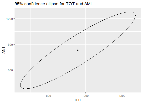
The dot in the center is our predicted values for TOT and AMI. The ellipse represents the uncertainty in this prediction. We're 95% confident the true mean values of TOT and AMI when GEN = 1 and AMT = 1200 are within the area of the ellipse. Notice also that TOT and AMI seem to be positively correlated. Predicting higher values of TOT means predicting higher values of AMI, and vice versa.
R session details
The analysis was done using the R Statistical language (v4.5.2; R Core Team, 2025) on Windows 11 x64, using the packages car (v3.1.3) and carData (v3.0.5).
References
- Fox J and Weisberg S (2011). An {R} Companion to Applied Regression, Second Edition. Thousand Oaks CA: Sage. URL: http://socserv.socsci.mcmaster.ca/jfox/Books/Companion
- Johnson R and Wichern D (2007). Applied Multivariate Statistical Analysis, Sixth Edition. Prentice-Hall.
- R Core Team (2025). R: A Language and Environment for Statistical Computing. R Foundation for Statistical Computing, Vienna, Austria. https://www.R-project.org/.
- Rudorfer MV (1982). “Cardiovascular Changes and Plasma Drug Levels after Amitriptyline Overdose.” Journal of Toxicology-Clinical Toxicology, 19, 67-71.
Clay Ford
Statistical Research Consultant
University of Virginia Library
October 27, 2017
Updated May 26, 2023
Update February 20, 2024 (changed function name)
For questions or clarifications regarding this article, contact statlab@virginia.edu.
View the entire collection of UVA Library StatLab articles, or learn how to cite.