
Whenever we are dealing with a dataset, we almost always run into a problem that may decrease our confidence in the results that we are getting - missing data! Examples of missing data can be found in surveys - where respondents intentionally refrained from answering a question, didn’t answer a question because it is not applicable to them, or simply forgot to give an answer. Or our dataset on trade in agricultural products for country-pairs over years could suffer from missing data as some countries fail to report their accounts for certain years. One important distinction to make here - when a country records 0 trade with another country, this doesn’t count as missing data. Missing data occurs when we have no information about that data point in the dataset because of missing information.
What should we do when we encounter missing data in our datasets? There are a couple of strategies you can employ in this case, but you have to be careful with what you choose, because all options have pros and cons:
- Listwise-deletion (also called Complete Case Analysis): You can choose to delete rows in your dataset that contains missing data (NAs, NaN, ., in whichever form they come). If the amount of missing data is very small, this might be the best way to go to ensure you are not biasing your analysis. However, deleting datapoints will nevertheless deprive you of important information, especially if your dataset is small. It will reduce your degrees of freedom in statistical analysis and force you to get rid of valid data points just because one column value is missing. Nevertheless, this is the most common approach in quantitative research to deal with missing data.
- Mean/median substitution: Another quick fix is to take the mean/median of the existing data points and substitute missing data points with the mean/median. This might look like a fine approach since it doesn’t change the mean of the dataset, but could cause bias in the analysis since it decreases variance (if you have a lot of missing data and you are replacing them with a fixed number). In reality, those datapoints could have been different numbers, which causes a decrease in variance.
- Multiple Imputation: This requires more work than the other two options. With this approach, rather than replacing missing values with a single value, we use the distribution of the observed data/variables to estimate multiple possible values for the data points. This allows us to account for the uncertainty around the true value, and obtain approximately unbiased estimates (under certain conditions). Moreover, accounting for uncertainty allows us to calculate standard errors around estimations, which in turn leads to a better sense of uncertainty for the analysis. This method is also more flexible since it can be applied to any kind of data and any kind of analysis, and the researcher has flexibility in deciding how many imputations are necessary for the data at hand.
In this blog post, I am going to talk about the third option - multiple imputation - to deal with missing values. Although there are several packages (mi developed by Gelman, Hill and others; hot.deck by Gill and Cramner, Amelia by Honaker, King, Blackwell) in R that can be used for multiple imputation, in this blog post I’ll be using the mice package, developed by Stef van Buuren. Before getting into the package details, I’d like to present some information on the theory behind multiple imputation, proposed by Rubin in 1976.
Rubin proposed a five-step procedure in order to impute the missing data.
- impute the missing values by using an appropriate model which incorporates random variation.
- repeat the first step 3-5 times.
- perform the desired analysis on each data set by using standard, complete data methods.
- average the values of the parameter estimates across the missing value samples in order to obtain a single point estimate.
- calculate the standard errors by averaging the squared standard errors of the missing value estimates. After this, the researcher must calculate the variance of the missing value parameter across the samples. Finally, the researcher must combine the two quantities in multiple imputation for missing data to calculate the standard errors.
Put in a simpler way, we a) choose values that keep the relationship in the dataset intact in place of missing values b) create independently drawn imputed (usually 5) datasets c) calculate new standard errors using variation across datasets to take into account the uncertainty created by these imputed datasets (Kropko et al. 2014)
Missing Data Assumptions
Rubin (1976) classified types of missing data in three categories: MCAR, MAR, MNAR
- MCAR: Missing Completely at Random - the reason for the missingness of data points are at random, meaning that the pattern of missing values is uncorrelated with the structure of the data. An example would be a random sample taken from the population: data on some people will be missing, but it will be at random since everyone had the same chance of being included in the sample.
- MAR: Missing at Random - the missingness is not completely random, but the propensity of missingness depends on the observed data, not the missing data. An example would be a survey respondent choosing not to answer a question on income because they believe the privacy of personal information. As seen in this case, the missing value for income can be predicted by looking at the answers for the personal information question.
- MNAR: Missing Not at Random - the missing is not random, it correlates with unobservable characteristics unknown to a researcher. An example would be social desirability bias in survey - where respondents with certain characteristics we can’t observe systematically shy away from answering questions on racial issues.
All multiple imputation techniques start with the MAR assumption. While MCAR is desirable, in general it is unrealistic for the data. Thus, researchers make the assumption that missing values can be replaced by predictions derived by the observable portion of the dataset. This is a fundamental assumption to make, otherwise we wouldn’t be able to predict plausible values of missing data points from the observed data.
Mice package: How the package works in theory
mice stands for Multivariate Imputation by Chained Equations. We use this package in order to replace missing values with plausible values to estimate more realistic regression coefficients that are not affected by missing values. The mice package allows us to create a number of imputed datasets that replace missing values with plausible values and conduct our analysis on these separate, complete datasets in order to obtain one regression coefficient.
There are two approaches to multiple imputation, implemented by different packages in R:
- Joint Multivariate Normal Distribution Multiple Imputation: The main assumption in this technique is that the observed data follows a multivariate normal distribution. Therefore, the algorithm that R packages use to impute the missing values draws values from this assumed distribution.
Ameliaandnormpackages use this technique. The biggest problem with this technique is that the imputed values are incorrect if the data doesn’t follow a multivariate normal distribution. - Conditional Multiple Imputation: Conditional MI, as indicated in its name, follows an iterative procedure, modeling the conditional distribution of a certain variable given the other variables. This technique allows users to be more flexible as a distribution is assumed for each variable rather than the whole dataset.
mice package uses Conditional MI in order to impute values in the dataset. The figure below depicts the three main steps to multiple imputation:
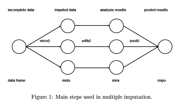
At the start of the process, we have a dataframe that contains missing values for several cases. What we would like to do is estimate a regression coefficient, for example to determine the effect of age on income, from this dataset. If there were no missing values, we would run an ols regression with lm() command, using our original dataset. Yet, we don’t want to delete all rows that have missing values from the dataset, as this will throw out important information and lower the number of observations in our data which will affect the statistical significance. Let’s say the number of observations in this dataset is 1,000. If we delete the rows with missing values, we will have 567 observations left. Therefore, we decide to impute the missing values.
As the first step, the mice command creates several complete datasets (in the figure above, n=3). It considers each missing value to follow a specific distribution, and draws from this distribution a plausible value to replace the missing value.
These complete datasets are stored in an object class called mids, short for multiply imputed dataset. These datasets are copies of the original dataframe except that missing values are now replaced with values generated by mice. Since these values are generated, they create additional uncertainty about what the real values of these missing data points are. We will need to factor in this uncertainty in the future as we are estimating the regression coefficients from these datasets.
Now that we have three complete datasets, the next step is to run an ols regression on all three datasets with 1,000 observations each (originally, we were going to run only one ols regression on the incomplete dataset with 567 observations). Using the with() function, we run the ols regression and obtain a different regression coefficient for each dataset. These three coefficients are different from each other because each dataset contains different imputed values, and we are uncertain about which imputed values are the correct ones. The analysis results are stored in a mira object class, short for multiply imputed repeated analysis.
Finally, we pool together the three coefficients estimated by the imputed dataset into one final regression coefficient, and estimate the variance using the pool() function. To obtain the final coefficient we just take the mean of three values. We calculate the variance of the estimated coefficient by factoring in the within (accounting for differences in predicted values from the dataset regarding each observation) and between (accounting for differences between three datasets) imputation variance.
Practical application of mice package with American National Election Survey 2012 (ANES) dataset
If you would like to follow along, here are the links to the datasets I use in this blog post:
- ANES 2012 - simplified version
- ANES 2012 - text supplement
- Chinese M&A dataset (taken from Rhodium Group)
In this blog post, we are going to use a sample from the American National Election Studies (ANES 2012) survey in order to impute the missing values. Most multiple imputation tutorials use small, simple datasets. While it is easier to showcase the basics of multiple imputation with these datasets, the datasets we work with for our research tend to be more complicated than that. Therefore, in this blog post, I try to highlight some complications regarding multiple imputation with relatively larger, more complicated data sets.
Analysis with Missing Values
First, we conduct our analysis with the ANES dataset using listwise-deletion. In this example, we are going to run a simple OLS regression, regressing sentiments towards Hillary Clinton in 2012 on occupation, party id, nationalism, views on China’s economic rise and the number of Chinese Mergers and Acquisitions (M&A) activity, 2000-2012, in a respondent’s state.
Dependent variable:
Sentiment towards Hillary Clinton: ANES Feeling Thermometer question on Hillary Clinton
Independent variables:
- Occupation (taken from ANES supplementary files): Dichotomous variables, 1 if the respondent works in manufacturing 0 if not
- Party ID: Continuous index that ranges from 0 (Strong Democrat) to 6 (Strong Republican)
- Nationalism: Continuous index that ranges from 0 (Not at all Important) to 4 (Extremely Important)
- Views on China’s economic rise: Dichotomous variable, 0 Good/No Effect 1 Bad
- The number of Chinese M&A activity: 2000-2012, Continuous variable that ranges from 0 to 60
library(dplyr)
library(mice)
library(foreign) # to import Stata DTA files
library(car)     # for recode

set.seed(145)
# Import ANES dataset
anesimp <- read.dta("anesimputation.dta",
                    convert.factors = FALSE, missing.type = TRUE)
# Dataset contains values <0. Code all of them as missing

for(i in 1:ncol(anesimp)){
  anesimp[,i] <- ifelse(anesimp[,i]<0, NA, anesimp[,i])
}
# Add occupation variable

anesocc <- read.csv("anesocc.csv",sep=";",na.strings=c("","NA"))
# Selecting occupation now and industry now variables
anesocc2 <- anesocc %>%
  dplyr::select(caseid, dem_occnow, dem_indnow)

# Coding any text that includes "manu" in it as respondent working in
# manufacturing, excluding manuver

# to address an 'invalid' string in row 3507
anesocc2$dem_occnow <- iconv(anesocc2$dem_occnow, from="UTF-8", to="")

anesocc2 <- anesocc2 %>%
  mutate(manuf = case_when((grepl("manu",dem_occnow)&!grepl("manuver",dem_occnow)) ~ 1,
                           grepl("manu",anesocc2$dem_indnow) ~ 1,
                           is.na(dem_occnow) ~ NA_real_,
                           is.na(dem_indnow) ~ NA_real_,
                           !is.na(dem_occnow) ~ 0,
                           !is.na(dem_indnow) ~ 0)
  )


anesocc2 <- anesocc2 %>%
  dplyr::select(manuf)

# combining by columns as they are sorted in the same order
anesimp <- cbind(anesimp,anesocc2)

# Merge M&A data

maimp <- read.dta("ma.dta")
anesimp <- merge(x=anesimp, y=maimp, by=c("sample_state"))

# Recode variables
anesimp$patriot_amident <- recode(anesimp$patriot_amident,
                                  "5=0; 4=1; 3=2; 2=3; 1=4")

anesimp$econ_ecnext_x <- recode(anesimp$econ_ecnext_x,
                                "1=0; 2=1; 3=2; 4=3; 5=4")

anesimp$pid_x <- recode(anesimp$pid_x,
                        "1=0; 2=1; 3=2; 4=3; 5=4; 6=5; 7=6")

anesimp$dem_edugroup_x <- recode(anesimp$dem_edugroup_x,
                                 "1=0; 2=1; 3=2; 4=3; 5=4")

# Treat manuf as a factor
anesimp$manuf <- as.factor(anesimp$manuf)


# Save the dataframe as another object so that we can use the original dataframe
# for multiple imputation
anesimpor <- anesimp

# Transform variables for regression
# Treat nationalism as continuous
anesimpor$patriot_amident <- as.numeric(anesimpor$patriot_amident)
# Treat party id as continuous
anesimpor$pid_x <- as.numeric(anesimpor$pid_x)
# Treat china_econ as dichotomous
anesimpor$china_econ <- recode(anesimpor$china_econ, "1=0; 3=0; 2=1")
anesimpor$china_econ <- as.factor(anesimpor$china_econ)

# Take the log of Chinese M&A variables - add a small number as variable
# contains 0s
anesimpor$LogMANO <- log(anesimpor$MANo+1.01)
# Treat party id as continuous

# Estimate an OLS regression

fitols <- lm(ft_hclinton ~ manuf + pid_x + patriot_amident +
               china_econ + LogMANO, data=anesimpor)

summary(fitols)
Call:
lm(formula = ft_hclinton ~ manuf + pid_x + patriot_amident +
    china_econ + LogMANO, data = anesimpor)

Residuals:
    Min      1Q  Median      3Q     Max
-86.972 -14.316   2.205  15.778  69.791

Coefficients:
                Estimate Std. Error t value Pr(>|t|)
(Intercept)      78.2653     1.4683  53.303  < 2e-16 ***
manuf1           -0.2387     3.1897  -0.075   0.9404
pid_x            -8.6788     0.1638 -52.970  < 2e-16 ***
patriot_amident   1.8372     0.3703   4.961 7.27e-07 ***
china_econ1      -3.6606     0.6997  -5.232 1.75e-07 ***
LogMANO           0.4896     0.2964   1.652   0.0987 .
---
Signif. codes:  0 ‘***’ 0.001 ‘**’ 0.01 ‘*’ 0.05 ‘.’ 0.1 ‘ ’ 1

Residual standard error: 22.85 on 4443 degrees of freedom
  (1465 observations deleted due to missingness)
Multiple R-squared:  0.4008,	Adjusted R-squared:  0.4001
F-statistic: 594.4 on 5 and 4443 DF,  p-value: < 2.2e-16
As we can see in the table above, 1,465 rows were deleted because one of these variables were missing. Our dataset contains 5,914 observations. This means that to conduct the regression, we had to throw away about 25% of our observations due to missingness. In this case, what we can do is use multiple imputation to replace missing values with plausible values depending on the structure of the dataset and distribution of variables. In this example, we will use mice package to implement the multiple imputation.
Preprocessing Data
Since we have already constructed our dataset to run the linear regression, we don’t need to do much preprocessing of the data in this step. In general, it is best to impute data in its rawest form possible, as any change could be derailing from its original distribution (such as creating a new variable based on existing variables, or any transformation of variables). One exception here is the manufacturing variable I’ve created based on open-ended text questions. I choose to create and code this variable, instead of imputing text as factor.
We include party identification and nationalism as continuous indices and views on China’s economic rise as a dichotomous variable. However, the first two in ANES are treated as ordered categorical and the latter is an unordered categorical variable. While we are imputing the dataset, it is important to keep the types of variables as they are, and determine different distributions for each variable according to their types.
# Use anesimp as the raw dataset

anesimp2 <- anesimp

# Treat variables as factors
anesimp2$patriot_amident <- as.factor(anesimp2$patriot_amident)
anesimp2$china_econ <- as.factor(anesimp2$china_econ)
anesimp2$pid_x <- as.factor(anesimp2$pid_x)
Pattern of Missing Data Exploration
Before moving on to determining the specifics of multiple imputation, we should first explore and see the pattern of missing data in our dataset.
p_missing <- unlist(lapply(anesimp2, function(x) sum(is.na(x))))/nrow(anesimp)
sort(p_missing[p_missing > 0], decreasing = TRUE)
          relig_ident_1st        iwrobspre_skintone
             0.6687521136              0.6628339533
       iwrobspre_interest         iwrobspre_levinfo
             0.6569157930              0.6567467027
         iwrobspre_intell          prevote_primvwho
             0.6567467027              0.6396685830
          gayrt_discrev_x      interest_whovote2008
             0.5285762597              0.2357118701
        prevote_intpresst             prevote_inths
             0.2336827866              0.1758539060
          prevote_intpres                     manuf
             0.1660466689              0.1511667230
            prevote_voted                china_econ
             0.1220831924              0.1180250254
             libcpre_self          inc_incgroup_pre
             0.1038214406              0.0879269530
                  ft_rvpc             dem2_cellpers
             0.0867433209              0.0722015556
          patriot_amident             congapp_job_x
             0.0713561042              0.0684815692
          prmedia_wkinews                   ft_dvpc
             0.0507270883              0.0483598241
        presapp_foreign_x             presapp_war_x
             0.0437943862              0.0405816706
            owngun_owngun               war_worthit
             0.0317889753              0.0307744335
             orientn_rgay          presapp_health_x
             0.0295908015              0.0272235374
           presapp_econ_x             wealth_stocks
             0.0262089956              0.0250253635
           campfin_banads             econ_ecnext_x
             0.0233344606              0.0233344606
            presapp_job_x         finance_finnext_x
             0.0231653703              0.0211362868
          preknow_senterm             presapp_track
             0.0199526547              0.0196144741
            ineq_incgap_x           trustgov_corrpt
             0.0196144741              0.0194453838
             usworld_stay               ineq_incgap
             0.0179235712              0.0165708488
                 aa_uni_x                    aa_uni
             0.0152181265              0.0145417653
           candaff_prdrpc           divgov_splitgov
             0.0143726750              0.0140344944
                aa_work_x          health_2010hcr_x
             0.0126817721              0.0123435915
           wealth_vachome         finance_finpast_x
             0.0116672303              0.0113290497
            candaff_hprpc          wealth_ownrental
             0.0113290497              0.0113290497
                   ft_rep              immig_checks
             0.0106526885              0.0103145079
         wealth_investbus               dem_age_r_x
             0.0103145079              0.0101454177
               war_terror         preknow_prestimes
             0.0099763274              0.0099763274
                   ft_dem            candaff_angrpc
             0.0098072371              0.0098072371
         usworld_stronger                    ft_rpc
             0.0098072371              0.0087926953
            econ_unpast_x            candaff_afrrpc
             0.0087926953              0.0084545147
           dem_edugroup_x              immig_policy
             0.0084545147              0.0079472438
          preknow_leastsp             prevote_primv
             0.0079472438              0.0072708827
            econ_ecpast_x            dem3_yearscomm
             0.0072708827              0.0072708827
           candaff_prddpc           happ_lifesatisf
             0.0069327021              0.0060872506
               econ_ecnow            candaff_angdpc
             0.0057490700              0.0055799797
             relig_import          preknow_medicare
             0.0054108894              0.0054108894
                   ft_gwb           preknow_sizedef
             0.0052417991              0.0052417991
           candaff_afrdpc      preswin_dutychoice_x
             0.0050727088              0.0050727088
            immig_citizen               dem_unionhh
             0.0050727088              0.0049036185
            dem_raceeth_x             dem3_passport
             0.0049036185              0.0049036185
              ft_hclinton             candaff_hpdpc
             0.0047345282              0.0045654379
              gun_control              dem3_ownhome
             0.0042272574              0.0042272574
                    pid_x        interest_voted2008
             0.0040581671              0.0037199865
             dem_nativity       relig_mastersummary
             0.0035508962              0.0028745350
                   ft_dpc            finance_finfam
             0.0025363544              0.0025363544
             health_smoke dem_empstatus_1digitfin_x
             0.0023672641              0.0021981738
           health_insured               health_self
             0.0020290835              0.0020290835
           gun_importance           prmedia_wkrdnws
             0.0020290835              0.0016909029
              dem_marital         prmedia_wkpaprnws
             0.0016909029              0.0013527224
          prmedia_wktvnws        interest_following
             0.0010145418              0.0008454515
              dem_veteran        interest_attention
             0.0006763612              0.0005072709
            dem2_numchild
             0.0005072709
The code above calculates what percent of data is missing. A simple look at this table warns us about several variables that have more than 25% missing - such as prevote_primvwho, iwrobspre_skintone and relig_ident_1st. It is useful to remove these variables from the dataset first as they might mess up the imputation. I also remove additional variables that are highly correlated with others that stop the imputation working otherwise (see Troubleshooting section for more information).
Looking at the table, we also see that some variables are character variables indicating state names. We have both sample_state and Statename serving the same purpose. I delete the Statename variable, and turn the sample_state character vector into a factor (see Troubleshooting for more information). I don’t create any new variables or conduct variable transformations at this point.
# Select out variables that could cause problems in the imputation process
anesimp2 <- anesimp2 %>%
  dplyr::select(-interest_whovote2008,-prevote_primvwho, -prevote_intpresst,
                -relig_ident_1st,-iwrobspre_skintone,-iwrobspre_levinfo,
                -iwrobspre_intell, -iwrobspre_interest,-gayrt_discrev_x,
                -Statename)

anesimp2$sample_state <- as.factor(anesimp2$sample_state)
At this step, we need to specify distributions for our to-be-imputed variables and determine which variables we would like to leave out of the imputation prediction process. We will extract information on the predictor matrix and imputation methods to change them.
The Predictor Matrix informs us which variables are going to be used to predict a plausible value for variables (1 means a variable is used to predict another variable, 0 otherwise). Since no variable can predict itself, the intersection of one variable with itself in the matrix takes the value 0. We can manually determine if we would like to leave certain variables out of prediction. In this case, I’d like to leave out the manufacturing variable I constructed, state indicators, and all the state-level variables I merged into the dataset when I merged in Chinese M&A variables.
The mice package assumes a distribution for each variable and imputes missing variables according to that distribution. Hence, it is important to correctly specify each of these distributions. mice automatically chooses distributions for variables. If we would like to change them, we can do it by changing the methods’ characteristics. Even though we are going to use variables such as patriot_amident and pid_x as continuous later on, I’ll specify their imputation methods suited for ordered categorical variables.
# We run the mice code with 0 iterations

imp <- mice(anesimp2, maxit=0)

# Extract predictorMatrix and methods of imputation

predM <- imp$predictorMatrix
meth <- imp$method

# Setting values of variables I'd like to leave out to 0 in the predictor matrix
predM[, c("sample_state")] <- 0
predM[, c("Total_mil")] <- 0
predM[, c("PriOwn_mil")] <- 0
predM[, c("GovValue_mil")] <- 0
predM[, c("PriOwn")] <- 0
predM[, c("GovOwn")] <- 0
predM[, c("MANo")] <- 0
predM[, c("manuf")] <- 0

# If you like, view the first few rows of the predictor matrix
# head(predM)

# Specify a separate imputation model for variables of interest

# Ordered categorical variables
poly <- c("patriot_amident", "pid_x")

# Dichotomous variable
log <- c("manuf")

# Unordered categorical variable
poly2 <- c("china_econ")

# Turn their methods matrix into the specified imputation models
meth[poly] <- "polr"
meth[log] <- "logreg"
meth[poly2] <- "polyreg"

meth
             sample_state       gender_respondent_x
                       ""                        ""
       interest_attention        interest_following
                    "pmm"                     "pmm"
       interest_voted2008           prmedia_wkinews
                    "pmm"                     "pmm"
          prmedia_wktvnws         prmedia_wkpaprnws
                    "pmm"                     "pmm"
          prmedia_wkrdnws             prevote_primv
                    "pmm"                     "pmm"
            prevote_voted           prevote_intpres
                    "pmm"                     "pmm"
            prevote_inths             congapp_job_x
                    "pmm"                     "pmm"
            presapp_track             presapp_job_x
                    "pmm"                     "pmm"
           presapp_econ_x         presapp_foreign_x
                    "pmm"                     "pmm"
         presapp_health_x             presapp_war_x
                    "pmm"                     "pmm"
                   ft_dpc                    ft_rpc
                    "pmm"                     "pmm"
                  ft_dvpc                   ft_rvpc
                    "pmm"                     "pmm"
              ft_hclinton                    ft_gwb
                    "pmm"                     "pmm"
                   ft_dem                    ft_rep
                    "pmm"                     "pmm"
           finance_finfam         finance_finpast_x
                    "pmm"                     "pmm"
        finance_finnext_x            health_insured
                    "pmm"                     "pmm"
         health_2010hcr_x               health_self
                    "pmm"                     "pmm"
             health_smoke            candaff_angdpc
                    "pmm"                     "pmm"
            candaff_hpdpc            candaff_afrdpc
                    "pmm"                     "pmm"
           candaff_prddpc            candaff_angrpc
                    "pmm"                     "pmm"
            candaff_hprpc            candaff_afrrpc
                    "pmm"                     "pmm"
           candaff_prdrpc              libcpre_self
                    "pmm"                     "pmm"
          divgov_splitgov            campfin_banads
                    "pmm"                     "pmm"
              ineq_incgap             ineq_incgap_x
                    "pmm"                     "pmm"
               econ_ecnow             econ_ecpast_x
                    "pmm"                     "pmm"
            econ_ecnext_x             econ_unpast_x
                    "pmm"                     "pmm"
     preswin_dutychoice_x          usworld_stronger
                    "pmm"                     "pmm"
             usworld_stay                     pid_x
                    "pmm"                    "polr"
              war_worthit                war_terror
                    "pmm"                     "pmm"
              gun_control            gun_importance
                    "pmm"                     "pmm"
             immig_policy             immig_citizen
                    "pmm"                     "pmm"
             immig_checks                    aa_uni
                    "pmm"                     "pmm"
                 aa_uni_x                 aa_work_x
                    "pmm"                     "pmm"
          trustgov_corrpt              relig_import
                    "pmm"                     "pmm"
      relig_mastersummary               dem_age_r_x
                    "pmm"                     "pmm"
              dem_marital            dem_edugroup_x
                    "pmm"                     "pmm"
              dem_veteran dem_empstatus_1digitfin_x
                    "pmm"                     "pmm"
              dem_unionhh             dem_raceeth_x
                    "pmm"                     "pmm"
             dem_nativity             dem2_numchild
                    "pmm"                     "pmm"
            dem2_cellpers            dem3_yearscomm
                    "pmm"                     "pmm"
             dem3_ownhome             dem3_passport
                    "pmm"                     "pmm"
            wealth_stocks            wealth_vachome
                    "pmm"                     "pmm"
         wealth_ownrental          wealth_investbus
                    "pmm"                     "pmm"
         inc_incgroup_pre             owngun_owngun
                    "pmm"                     "pmm"
             orientn_rgay         preknow_prestimes
                    "pmm"                     "pmm"
          preknow_sizedef           preknow_senterm
                    "pmm"                     "pmm"
         preknow_medicare           preknow_leastsp
                    "pmm"                     "pmm"
          happ_lifesatisf           patriot_amident
                    "pmm"                    "polr"
               china_econ             sample_stfips
                "polyreg"                        ""
            sample_region                     manuf
                       ""                  "logreg"
                     MANo                    GovOwn
                       ""                        ""
                   PriOwn              GovValue_mil
                       ""                        ""
               PriOwn_mil                 Total_mil
                       ""                        ""
As we can see above, our variables of interest are now configured to be imputed with the imputation method we specified. Empty cells in the method matrix mean those variables will not be imputed. Variables with no missing values are set to be empty. We can also manually set variables to not be imputed using the syntax meth[variable] <- "". For more information on additional imputation methods, see the mice help page.
Now that we are ready for multiple imputation, we can start the process by typing the code below. Our dataset consists of 5,914 rows and 106 variables, so this will probably take several minutes, or more, depending on the power of your computer.
# With this command, we tell mice to impute the anesimp2 data, create 5
# datasets, use predM as the predictor matrix and don't print the imputation
# process. If you would like to see the process, set print as TRUE

imp2 <- mice(anesimp2, maxit = 5,
             predictorMatrix = predM,
             method = meth, print =  FALSE)
We now have 5 imputed datasets. Across all datasets, non-missing values are the same. The imputation created 5 datasets with different plausible values for missing values. You can look at imputed datasets and values with the following commands:
# Look at head and tail of imputed values for china_econ variable
head(imp2$imp$china_econ)
   1 2 3 4 5
4  3 3 2 3 2
6  3 2 2 2 2
7  2 2 3 3 2
17 2 1 1 3 1
26 3 3 2 2 2
36 2 2 2 3 2
tail(imp2$imp$china_econ)
     1 2 3 4 5
5861 2 1 1 1 2
5868 2 2 2 2 1
5871 2 2 2 3 3
5876 1 1 3 1 1
5893 1 2 2 2 3
5902 2 2 2 1 2
# Can also extract the first imputed, complete dataset and look at the first
# rows using the complete function

# anescomp <- mice::complete(imp2, 1)
# head(anescomp)
Finally, we need to run the regression on each of the five datasets and pool the estimates together to get average regression coefficients and correct standard errors. The with function in the mice package allows us to do this.
# First, turn the datasets into long format
anesimp_long <- mice::complete(imp2, action="long", include = TRUE)

# Convert two variables into numeric
anesimp_long$patriot_amident <- with(anesimp_long,
                                     as.integer(anesimp_long$patriot_amident))
anesimp_long$pid_x <- with(anesimp_long,
                           as.integer(anesimp_long$pid_x))

# Take log of M&A variable
anesimp_long$LogMANO<-log(anesimp_long$MANo+1.01)

# Convert back to mids type - mice can work with this type
anesimp_long_mids<-as.mids(anesimp_long)
# Regression


fitimp <- with(anesimp_long_mids,
               lm(ft_hclinton ~ manuf + pid_x +
                    patriot_amident + china_econ + LogMANO))

summary(pool(fitimp))
                  estimate std.error   statistic         df      p.value
(Intercept)     85.2463594 1.7199020  49.5646605  533.92817 0.000000e+00
manuf1          -2.1889267 3.0489110  -0.7179372   38.15083 4.728247e-01
pid_x           -8.3825919 0.1460527 -57.3942947 2978.97122 0.000000e+00
patriot_amident  1.8537042 0.3364319   5.5098947  410.25972 3.744069e-08
china_econ2     -4.9288737 0.8754884  -5.6298558   74.40750 1.887622e-08
china_econ3     -2.3493172 0.9941761  -2.3630795  177.40494 1.815637e-02
LogMANO          0.5511566 0.2578248   2.1377176 5838.81197 3.258108e-02
The pooled coefficients from the imputed datasets gave us more or less similar results as we got with the listwise-deletion technique. P-values obtained from imputed datasets are also similar, except for one variable - log of Chinese M&A. After imputation, we observe a statistically significant effect of Chinese M&As on positive feeling towards Hillary Clinton. This effect was only significant at 90% confidence level using the listwise deletion technique. This shows that multiple imputation can make a difference, but it is always useful to check, re-impute, and do sensitivity analyses in order to make sure that the imputation doesn’t shed light on a false effect.
Troubleshooting
Now that we have covered the basics of multiple imputation, I’d like to finish my blog post with various problems I’ve encountered during the process and how to possibly overcome these problems.
- Character vectors in dataset: Multiple imputation doesn’t deal well with character vectors in the dataset. One possible solution is to delete the character vectors, but if you would like to impute them or use them for a multilevel model after imputation, this solution is not practical. You can either,
- Get rid of the character vector
- Convert the character vector into a factor
- High proportions of missing data in variables: Multiple imputation algorithms might not like to include variables that have missing values in high proportions. While you are in the data exploration stage, it might be useful to eliminate variables with more than 50% missing from the imputation process.
- High multicollinearity: Multiple imputation doesn’t like variables that are highly correlated with each other. In most cases, the mice algorithm will leave these variables out of the imputation process. However, in some cases, multiple imputation might fail to start from the beginning. If the code is giving you an error, it might be useful to run the imputation with only a subset of variables, and keep increasing the number of variables included until you find the problematic variable. If you set
print=TRUE, you will most likely see where the algorithm is having trouble as it will stop working while imputing that variable. - Missing values after imputation: Always check how your variables are imputed by inpecting the
impelement in the mids object (For example, as we did earlier:head(imp2$imp$china_econ)). If you still see missing values after imputation, this means the algorithm didn’t work as intended. There shouldn’t be huge differences between your analysis pre-imputation and after-imputation, unless missing values are highly affecting your analysis (in that case, it might be useful to think about other strategies to collect more data). I’d suggest you impute the whole dataset, rather than only the variable of interest. - Non-missing value variables: If you have variables with no missing values, you’ll most likely have to exclude them from the imputation process. This especially causes problems if your dataset is hierarchically ordered, like the one in this example. All state-level predictors needed to be excluded from imputation as no values were missing from these variables.
R session details
The analysis was done using the R Statistical language (v4.5.1; R Core Team, 2025) on Windows 11 x64, using the packages car (v3.1.3), carData (v3.0.5), foreign (v0.8.90), mice (v3.18.0) and dplyr (v1.1.4).
References
- Groothuis-Oudshoorn, K., and S. Van Buuren. (2011). “Mice: multivariate imputation by chained equations in R.” Journal of Statistical Software 45, no. 3: 1-67.
- Kropko, Jonathan, Ben Goodrich, Andrew Gelman, and Jennifer Hill. (2014). “Multiple imputation for continuous and categorical data: Comparing joint multivariate normal and conditional approaches.” Political Analysis 22, no. 4.
- Rubin, Donald B. (1976). “Inference and missing data.” Biometrika 63, no. 3: 581-592.
- Van Buuren, Stef. (2018). Flexible imputation of missing data. Chapman and Hall/CRC.
- Zhang Z. (2015). “Missing data exploration: highlighting graphical presentation of missing pattern.” Annals of Translational Medicine, 3(22), 356.
- The American National Election Studies 2012 (www.electionstudies.org). These materials are based on work supported by the National Science Foundation under grant numbers SES 1444721, 2014-2017, the University of Michigan, and Stanford University
- Chinese Investment Monitor, Rhodium Group. Link
Aycan Katitas
StatLab Associate
University of Virginia Library
May 1, 2019
For questions or clarifications regarding this article, contact statlab@virginia.edu.
View the entire collection of UVA Library StatLab articles, or learn how to cite.