
Multinomial logit models allow us to model membership in a group based on known variables. For example, the operating system preferences of a university’s students could be classified as “Windows,” “Mac,” or “Linux.” Perhaps we would like to better understand why students choose one OS versus another. We might want to build a statistical model that allows us to predict the probability of selecting an OS based on information such as sex, major, financial aid, and so on. Multinomial logit modeling allows us to propose and fit such models.
It’s important to note that multinomial logit models are best suited for nominal categories. These are categories with no natural ordering. The example presented above has no natural ordering. Despite the opinions of some computer users, Linux is not measurably “higher” or “lower” than Windows, nor is Mac “higher” or “lower” than Linux. They are distinct groups. Examples of ordered categories include sizes, pain scales, and age groups. These are categories in which one level might be considered greater than or less than an adjacent category. A common approach to modeling ordered categories is the ordered logit model, also known as the proportional odds model. For more information, see our related post, Fitting and Interpreting a Proportional Odds Model.
To illustrate multinomial logit models, we’ll use the R statistical programming environment and data on alligator food choice from the text An Introduction to Categorical Data Analysis by Alan Agresti (1996, p. 207). The data contain information on 59 alligators sampled from a lake in Florida. It has the length of the alligator in meters and the primary food type found in the alligator’s stomach. The food type was classified into three categories: "Fish", "Invertebrate", and "Other". Of interest is whether or not the length of an alligator is associated with the primary food type. Does knowing the length of an alligator give us some indication about its primary food type? If so, how is length associated with the choice of food type?
Let’s read in the data and examine it. (The code below should work for you if have an active internet connection.) Notice we make the food column a factor and set the reference (or baseline) level to “Other” by placing it first in the levels and labels arguments to factor(). We’ll explain why we do this in a bit.
gators <- read.csv('https://static.lib.virginia.edu/statlab/materials/data/table_8-1.csv')
gators$food <- factor(gators$food,
                      levels = c("O", "F", "I"),
                      labels = c("Other", "Fish", "Invertebrates"))
Looking at the counts and proportions, we see there is certainly variability between the food groups.
# counts
table(gators$food)
          Other          Fish Invertebrates
              8            31            20
# proportions
prop.table(table(gators$food))
          Other          Fish Invertebrates
      0.1355932     0.5254237     0.3389831
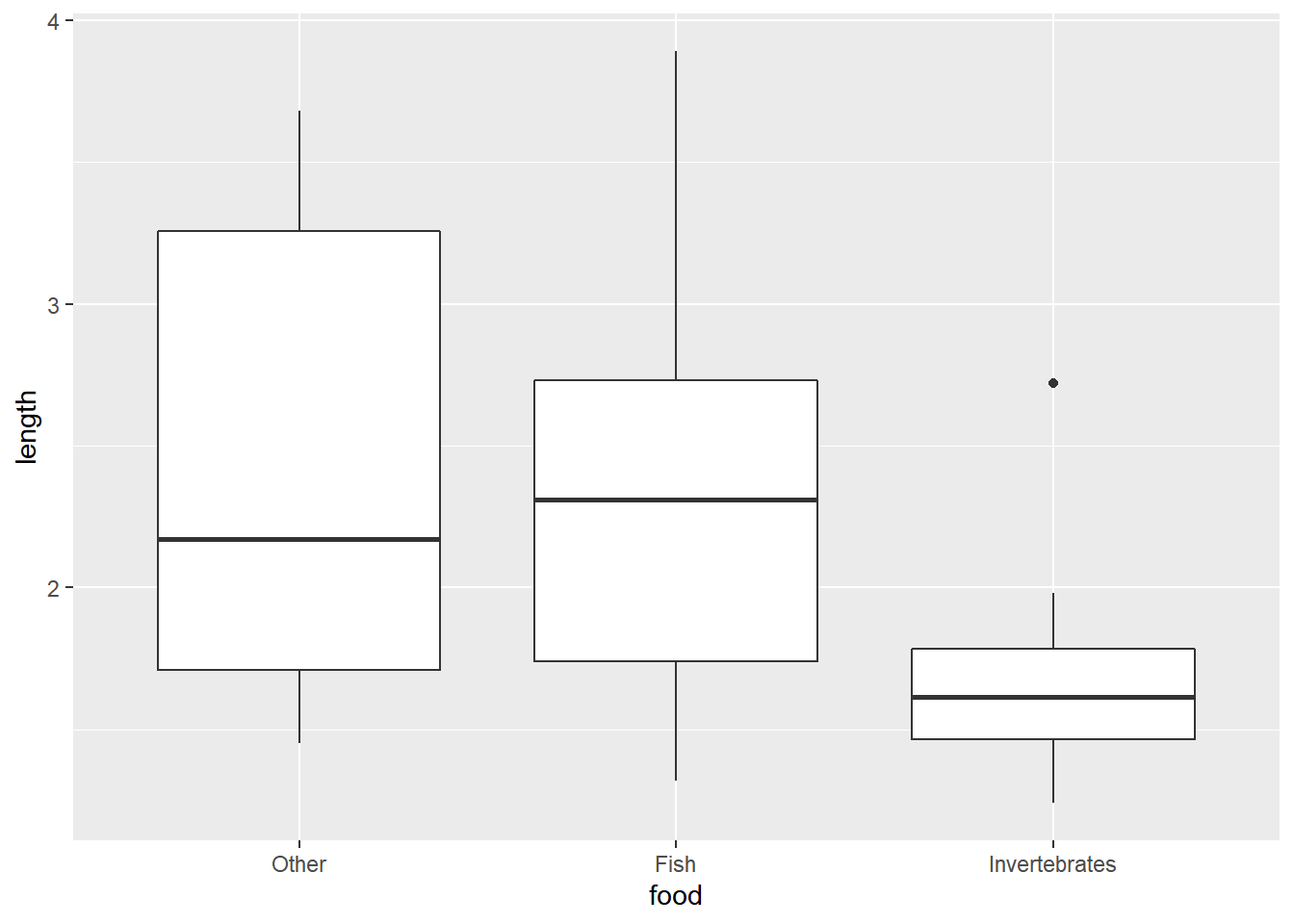
We can also explore the data visually using the ggplot2 package. First we make a boxplot of length by food choice.
library(ggplot2)
ggplot(gators) +
  aes(x = food, y = length) +
  geom_boxplot()
Next we make a one-dimensional scatter plot of length by food choice. Notice how we use position_jitter() to randomly scatter the points in a horizontal direction so they’re not overplotted.
ggplot(gators) +
  aes(y = length, x = food) +
  geom_point(position = position_jitter(width = 0.1, height = 0))
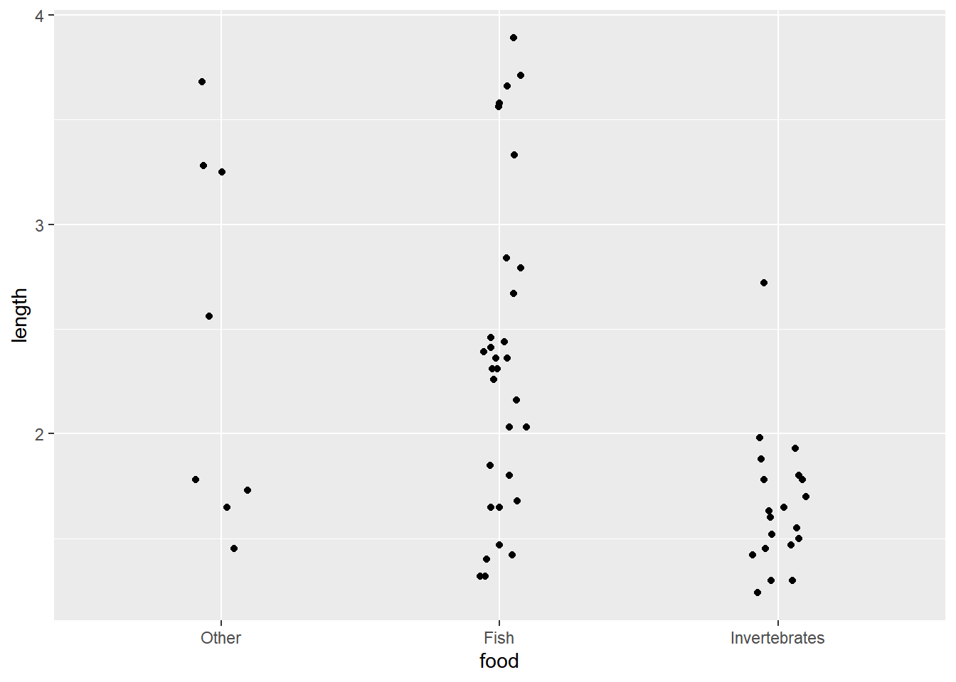
In both plots it seems smaller alligators are more likely to eat primarily invertebrates while bigger alligators are more likely to eat fish. It’s hard to infer much about the "Other" category, since we only have 8 observations which appear uniformly scattered over the range of data.
So we can see there appears to be some relationship between length and food choice, but how can we quantify it? How does primary food choice change as length changes? This is where multinomial logit modeling comes in.
In R, we can use the nnet package that comes installed with base R. It has the multinom() function which fits multinomial logit models via neural networks. Don’t worry, you don’t need to know anything about neural networks to use the function. In fact it works much like the workhorse modeling functions, lm() and glm().
To fit our model, we specify food to be modeled as a function of length using food ~ length. We specify data = gators so the function knows where to find the food and length variables. Finally, we specify Hess = TRUE to save something called the Hessian matrix, which is required to calculate coefficient standard errors, and we set trace = FALSE to suppress the printing of convergence progress.
library(nnet)
m <- multinom(food ~ length, data = gators,
              Hess = TRUE, trace = FALSE)
After fitting the model, we can use the summary() function to see coefficient estimates along with standard errors and test statistics. To see the Wald test statistics, we need to also set Wald.ratios = TRUE. We explain what those are below.
summary(m, Wald.ratios = TRUE)
Call:
  multinom(formula = food ~ length, data = gators, Hess = TRUE,
      trace = FALSE)

  Coefficients:
                (Intercept)     length
  Fish             1.617952 -0.1101836
  Invertebrates    5.697543 -2.4654695

  Std. Errors:
                (Intercept)    length
  Fish             1.307291 0.5170838
  Invertebrates    1.793820 0.8996485

  Value/SE (Wald statistics):
                (Intercept)     length
  Fish             1.237637 -0.2130865
  Invertebrates    3.176206 -2.7404808

  Residual Deviance: 98.34124
  AIC: 106.3412
The output is a little different from what you may be accustomed to seeing. In the "Coefficients" section, we're basically seeing two models, one modeling the predictive effect of length on the log odds that an alligator prefers fish to other, and the other modeling the predictive effect of length on the log odds that an alligator prefers invertebrates to other. This is why multinomial logit models are sometimes called baseline logit models. They model each category relative to some baseline level. In this case, the baseline level is “Other”, which we specified when we set the food variable as a factor above. In general, if you have J categories, you will have J-1 baseline logit models.
The next section provides standard errors of the coefficient estimates. These quantify uncertainty about the estimates. For example, the length coefficient for the "Invertebrates" model is -2.46 with a standard error of 0.89. The smaller the standard error in relation to the coefficient, the more precise the estimate. The section following the standard errors, Wald statistics, presents the ratio of the coefficients to the standard errors. The farther away the ratio is from 0, the more precise the estimate and the more likely it’s either positive or negative. This is no different from the output of other regression models. It’s just presented differently due to the fact we’re summarizing two models.
The summary() method for multinom() does not report p-values. However, that’s no hindrance to making inference about the “significance” of the coefficients. Wald statistics larger than 2 provide evidence that effects are reliably positive or negative. If you must report p-values, you’ll have to calculate them manually. Here’s one way using the standard normal approximation:
s <- summary(m, Wald.ratios = TRUE)
p <- 2 * pnorm(abs(s$Wald.ratios), lower.tail = FALSE)
p
                (Intercept)      length
  Fish          0.215850665 0.831259475
  Invertebrates 0.001492149 0.006134937
Despite their ubiquity, p-values don’t tell us anything about the size or direction of coefficients. They simply tell us the probability of our sample producing a test statistic (in this case, a Wald ratio) that far away from 0 (or farther) if the statistic really was 0.
Interpreting coefficients in logit models is difficult. The only thing that’s easy is determining whether or not the coefficient is positive or negative. For example, the length coefficient for the "Invertebrates" model is negative (-2.46) and has a large Wald statistic (greater than 2). It appears that the longer an alligator is, the less likely it is to eat invertebrates instead of "other." But that’s nothing we couldn’t have figured out from just looking at our exploratory plots.
The coefficient of -2.46 says that each additional meter of length reduces the log odds of choosing invertebrates over "other" by -2.46. Unfortunately, humans don’t think in terms of log odds. It can be shown that exponentiating the coefficient produces an odds ratio, which is a little easier to understand. Here we use the coef() function to extract the coefficients from the model, use indexing brackets to specify we want the length coefficient for the “Invertebrate vs. Other" model, and then use the exp() function to exponentiate.
exp(coef(m)['Invertebrates','length'])
[1] 0.08496894
The odds ratio is about 0.08. One way to interpret this is to imagine two groups of alligators, one that has gators 2 meters long (x) and another that has gators 3 meters long (x + 1). For alligators that are 3 meters long, the estimated odds that their food choice is invertebrate rather than "other" is (1 - 0.08) 92% less than the odds for alligators that are 2 meters in length. This interpretation is the same no matter the value of x. Obviously, you should choose a value in the range of your data.
Both the coefficient and odds ratio are just point estimates. Given a different sample, we would likely get different values. To get a sense of the range of values we might get with repeated samples and models, we can calculate 95% confidence intervals using the confint() function.
confint(m)
  , , Fish

                   2.5 %    97.5 %
  (Intercept) -0.9442917 4.1801963
  length      -1.1236492 0.9032821

  , , Invertebrates

                  2.5 %     97.5 %
  (Intercept)  2.181720  9.2133667
  length      -4.228748 -0.7021908
The confidence interval for the length coefficient in the "Invertebrates" model is about (-4.23, -0.70). We can exponentiate that to get a confidence interval for the odds ratio. Below we use indexing brackets to pull out the confidence interval from the 3-dimensional array that confint(m) returns. The first dimension is rows, so we specify “length”. The second dimension is columns, but we leave it blank to indicate we want all columns. The third dimension is the model, and we specify we want the “Invertebrates” model. Finally we exponentiate.
exp(confint(m)['length',,'Invertebrates'])
       2.5 %     97.5 %
  0.01457062 0.49549858
This suggests that if we repeatedly sampled and modeled alligators from this lake, 95% of the time we would get odds ratios ranging in value from about 0.01 to 0.50.
What if we wanted to estimate the odds ratio that a gator prefers fish to invertebrates? We could refit the model with "Invertebrate" as the baseline level and use the same process just described. Alternatively, we can subtract the "Invertebrates" coefficients from the "Fish" coefficients as follows:
exp((coef(m)[1,] - coef(m)[2,])["length"])
    length
  10.54114
For alligators of length x + 1 meters, the estimated odds that the food choice is fish rather than invertebrates is about 10 times the estimated odds for alligators of length x.
Expressing these relationships in odds ratios is a little better than using log odds, but it's still not ideal for many people. Probability is something that is more natural to work with. Fortunately, we can use multinomial logit models to estimate probabilities. For example, what’s the probability an alligator that is 2.5 meters long prefers fish? The predict() function allows us to easily estimate this. We just need to use the newdata argument to provide the model input as a data frame and set the type='probs' argument to ensure we get probabilities.
predict(m, newdata = data.frame(length = 2.5), type = 'probs')
          Other          Fish Invertebrates
      0.1832844     0.7017184     0.1149973
Our model estimates that a gator 2.5 meters long has 70% probability of preferring fish. Notice the predict() function also returns estimated probabilities for the two other categories as well. Like the coefficients and odds ratios, the probabilities are just point estimates. Once again confidence intervals help us understand the uncertainty in our estimated probabilities.
A convenient function for obtaining confidence intervals for probabilities is the ggeffect() function from the ggeffects package. Here we use it to get estimated probabilities and confidence intervals for lengths ranging from 1 to 4 in steps of 0.5. We do that by specifying terms = "length[1:4,by=0.5]".
library(ggeffects)
ggeffect(m, terms = "length[1:4,by=0.5]")
  # Predicted probabilities of food
  # x = length

  # Response Level = Other

     x | Predicted |   SE |       95% CI
  --------------------------------------
  1.00 |      0.03 | 0.91 | [0.01, 0.17]
  1.50 |      0.08 | 0.59 | [0.03, 0.22]
  2.00 |      0.14 | 0.44 | [0.06, 0.28]
  2.50 |      0.18 | 0.40 | [0.09, 0.33]
  3.00 |      0.21 | 0.50 | [0.09, 0.41]
  4.00 |      0.23 | 0.91 | [0.05, 0.65]

  # Response Level = Fish

     x | Predicted |   SE |       95% CI
  --------------------------------------
  1.00 |      0.15 | 0.69 | [0.04, 0.40]
  1.50 |      0.34 | 0.38 | [0.19, 0.52]
  2.00 |      0.56 | 0.32 | [0.41, 0.71]
  2.50 |      0.70 | 0.38 | [0.53, 0.83]
  3.00 |      0.75 | 0.47 | [0.55, 0.88]
  4.00 |      0.76 | 0.90 | [0.35, 0.95]

  # Response Level = Invertebrates

     x | Predicted |   SE |       95% CI
  --------------------------------------
  1.00 |      0.82 | 0.69 | [0.54, 0.95]
  1.50 |      0.58 | 0.38 | [0.40, 0.75]
  2.00 |      0.30 | 0.36 | [0.17, 0.47]
  2.50 |      0.11 | 0.66 | [0.03, 0.32]
  3.00 |      0.04 | 1.03 | [0.01, 0.23]
  4.00 |      0.00 | 1.80 | [0.00, 0.11]
Standard errors are on link-scale (untransformed).
Looking in the table, under the section “Response Level = Fish”, we see the 95% confidence interval on the estimated probability of 0.7 is (0.53, 0.83). We can also save this result and use it to visualize all the estimated probabilities and their associated confidence bands as an effect plot. First we save the result as eff. Next we use the ggplot() function and specify we want length (x) on the x-axis, predicted probabilities (predicted) on the y-axis, and all colors and fill aesthetics mapped to food group (response.level). Then we draw a line for the predicted values and a ribbon for the lower and upper confidence limits (conf.low and conf.high).
eff <- ggeffect(m, terms = "length[1:4,by=0.5]")
ggplot(eff) +
  aes(x = x, y = predicted, fill = response.level, color = response.level) +
  geom_line() +
  geom_ribbon(aes(ymin = conf.low, ymax = conf.high), alpha = 1/3) +
  labs(x = 'Length of Alligator', y = 'Predicted Probability') +
  ylim(c(0, 1))
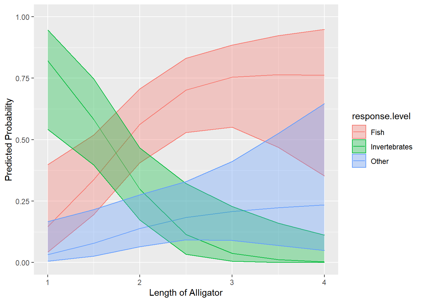
Now we clearly see that bigger alligators prefer fish, especially when they are larger than 2 meters. Likewise smaller alligators seem to prefer invertebrates, probably because they may not be big enough to easily consume fish. We can also see there is a great deal of uncertainty in predicted probabilities of food category beyond 3 meters of length. As expected, the predicted probability of the "other" food group as a function of length is inconclusive since we only had 8 gators in that group who widely varied in their lengths.
Finally we sometimes want to test whether a predictor variable is adding any value to a model. In this case we only have one predictor, length, and we’ve shown through Wald statistics and confidence intervals that it seems to be useful in understanding an alligator’s primary food choice. However, if we wanted to formally test whether a model with length is better than the null model with just an intercept, we can carry out a likelihood ratio test using the Anova() function in the car package.
library(car)
Anova(m)
  Analysis of Deviance Table (Type II tests)

  Response: food
         LR Chisq Df Pr(>Chisq)
  length   16.801  2  0.0002248 ***
  ---
  Signif. codes:  0 '***' 0.001 '**' 0.01 '*' 0.05 '.' 0.1 ' ' 1
The result is a test of whether or not the length coefficient in both baseline logit models is plausibly 0. The null is that a model with just an intercept is equally as good as a model with an intercept and length. (An intercept-only model is the same as simply using the observed proportions in each food category as a basis for making predictions about an alligator’s food choice.) The small p-value (p = 0.0002248) provides evidence against the null and leads us to keep length in our model.
R session details
The analysis was done using the R Statistical language (v4.5.1; R Core Team, 2025) on Windows 11 x64, using the packages car (v3.1.3), carData (v3.0.5), ggeffects (v2.3.1), nnet (v7.3.20) and ggplot2 (v3.5.2).
References
- Agresti, A. (1996). An introduction to categorical data analysis. Wiley.
- Bilder, C., & Loughin, T. (2015). Analysis of categorical data with R. CRC Press.
- Friendly, M, & Meyer, D. (2016). Discrete data analysis with R. CRC Press.
Clay Ford
Statistical Research Consultant
University of Virginia Library
September 1, 2020
For questions or clarifications regarding this article, contact statlab@virginia.edu.
View the entire collection of UVA Library StatLab articles, or learn how to cite.