Getting Started with Hurdle Models

Hurdle Models are a class of models for count data that help handle excess zeros and overdispersion. To motivate their use, let's look at some data in R. The following data come with the AER package. It is a sample of 4,406 individuals, aged 66 and over, who were covered by Medicare in 1988. One of the variables the data provide is number of physician office visits. Let's say we wish to model the number of visits (a count) by some of the other variables in the data set. To get started, we need to load the data. You may also need to install the AER package.

# Install the AER package (Applied Econometrics with R)
# install.packages("AER")

# load package 
library(AER)

# load the data
data("NMES1988")         

# select certain columns; Col 1 is number of visits
nmes <- NMES1988[, c(1, 6:8, 13, 15, 18)]  

With our data loaded, let's see how the number of visits is distributed. We do that by first counting up the number of occurrences for each visit and then plotting the table.

plot(table(nmes$visits))

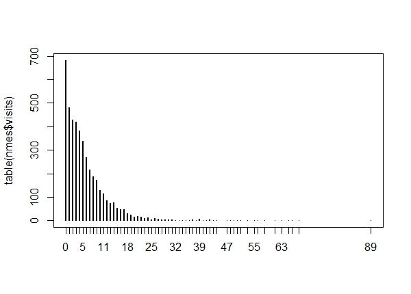
Close to 700 people had 0 visits. And a few people had more than 50 visits. We can count these up if we like:

sum(nmes$visits < 1)

[1] 683

sum(nmes$visits > 50)

[1] 13

A common approach to modeling count data is Poisson regression. When performing Poisson regression we're assuming our count data follow a Poisson distribution with a mean conditional on our predictors. Let's fit a Poisson model to our data, regressing number of visits on all other predictors, which include gender, number of years of education, number of chronic conditions, number of hospital stays, private insurance indicator and health (a 3-level categorical variable). Below, the syntax visits ~ . says to regress visits on all other variables in the nmes data frame. This analysis (and several others) is presented in the examples that accompany the NMES1998 data in the AER package.

mod1 <- glm(visits ~ ., data = nmes, family = "poisson")

Now let's see how many zeros this model predicts and compared to what we observed. We can do that by first predicting the expected mean count for each observation, and then using those expected mean counts to predict the probability of a zero count. Then we can sum those expected probabilities to get an estimate of how many zero counts we might expect to see.

# predict expected mean count
mu <- predict(mod1, type = "response")

# sum the probabilities of a 0 count for each mean
exp <- sum(dpois(x = 0, lambda = mu))

# predicted number of 0's
round(exp) 

[1] 47

# observed number of 0's
sum(nmes$visits < 1)

[1] 683          

We see that we're severely underfitting zero counts. We observed almost 700 zero counts but our model only predicts about 47. This is where the hurdle model comes in. The hurdle model is a two-part model that specifies one process for zero counts and another process for positive counts. The idea is that positive counts occur once a threshold is crossed, or put another way, a hurdle is cleared. If the hurdle is not cleared, then we have a count of 0. The first part of the model is typically a binary logit model. This models whether an observation takes a positive count or not. The second part of the model is usually a truncated Poisson or Negative Binomial model. Truncated means we're only fitting positive counts. If we were to fit a hurdle model to our nmes data, the interpretation would be that one process governs whether a patient visits a doctor or not, and another process governs how many visits are made. Let's go ahead and do that. The pscl package provides a function, hurdle, for fitting hurdle models. It works pretty much like other model fitting functions in R, except it allows you to fit different models for each part. To begin we'll fit the same model for both parts. First we install the package (in case you don't already have it), load the package, and then fit a hurdle model. By default the zero-count process is "binomial" (ie, binary logistic regression) and the positive-count process is "poisson". Notice we can specify those distributions explicitly using the dist and zero.dist arguments. Once again, the syntax visits ~ . says to regress visits on all other variables in the nmes data frame, except now it means we're doing it for both zero-count and positive-count processes.

# install.packages("pscl")
library(pscl)
mod.hurdle <- hurdle(visits ~ ., data = nmes)
# same as this:
# mod.hurdle <- hurdle(visits ~ ., data = nmes, dist = "poisson", 
                          zero.dist = "binomial")
summary(mod.hurdle)

					  
Call:
hurdle(formula = visits ~ ., data = nmes)

Pearson residuals:
    Min      1Q  Median      3Q     Max 
-5.4144 -1.1565 -0.4770  0.5432 25.0228 

Count model coefficients (truncated poisson with log link):
                 Estimate Std. Error z value Pr(>|z|)    
(Intercept)      1.406459   0.024180  58.167  < 2e-16 ***
hospital         0.158967   0.006061  26.228  < 2e-16 ***
healthpoor       0.253521   0.017708  14.317  < 2e-16 ***
healthexcellent -0.303677   0.031150  -9.749  < 2e-16 ***
chronic          0.101720   0.004719  21.557  < 2e-16 ***
gendermale      -0.062247   0.013055  -4.768 1.86e-06 ***
school           0.019078   0.001872  10.194  < 2e-16 ***
insuranceyes     0.080879   0.017139   4.719 2.37e-06 ***
Zero hurdle model coefficients (binomial with logit link):
                 Estimate Std. Error z value Pr(>|z|)    
(Intercept)      0.043147   0.139852   0.309 0.757688    
hospital         0.312449   0.091437   3.417 0.000633 ***
healthpoor      -0.008716   0.161024  -0.054 0.956833    
healthexcellent -0.289570   0.142682  -2.029 0.042409 *  
chronic          0.535213   0.045378  11.794  < 2e-16 ***
gendermale      -0.415658   0.087608  -4.745 2.09e-06 ***
school           0.058541   0.011989   4.883 1.05e-06 ***
insuranceyes     0.747120   0.100880   7.406 1.30e-13 ***
---
Signif. codes:  0 '***' 0.001 '**' 0.01 '*' 0.05 '.' 0.1 ' ' 1 

Number of iterations in BFGS optimization: 14 
Log-likelihood: -1.613e+04 on 16 Df

In our summary we get output for two different models. The first section of output is for the positive-count process. The second section is for the zero-count process. We can interpret these just as we would for any other model. Having fit a hurdle model, how many 0 counts does it predict? This is a little trickier to extract. First we use the predict function with type = "prob". This returns a predicted probability for all possible observed counts for each observation. In this case, that returns a 4406 x 90 matrix. That's 4406 rows for each observation, and 90 possible counts. The first column contains the predicted probabilities for getting a 0 count. As before we can sum those probabilities to get an expected number of 0 counts.

sum(predict(mod.hurdle, type = "prob")[,1])

[1] 683

We get 683, which happens to be the number of zeros in the observed data. This is by design. The hurdle model will always predict the same number of zeros as we observed. We can also predict the expected mean count using both components of the hurdle model. The mathematical expression for this is $$E[y | \textbf{x}] = \frac{1 - f_{1}(0|\textbf{x})}{1 - f_{2}(0|\textbf{x})} \mu_{2}(\textbf{x}) $$ This says the expected count (y) given our predictors (x) is a product of two things: a ratio and a mean. The ratio is the probability of a non-zero in the first process divided by the probability of a non-zero in the second untruncated process. The f symbols represents distributions. Recall these are logistic and Poisson, respectively, by default but can be others. The mean is the expected count of the positive-count process. For more details on this expression, truncated counts, and hurdle models in general, see Cameron and Trivedi (2013). We can use the predict function to get these expected mean counts by setting type = "response", which is the default.

# First 5 expected counts
predict(mod.hurdle, type = "response")[1:5]

        1         2         3         4         5 
 5.981262  6.048998 15.030446  7.115653  5.493896 

Referring to the expression above, we can also extract the ratio and the mean by specifying a different type argument:

# ratio of non-zero probabilities
predict(mod.hurdle, type = "zero")[1:5]

        1         2         3         4         5 
0.8928488 0.9215760 0.9758270 0.8728787 0.9033806 

# mean of positive-count process
predict(mod.hurdle, type = "count")[1:5]

        1         2         3         4         5 
 6.699076  6.563754 15.402777  8.151937  6.081485

And of course we can multiply them and confirm they equal the expected hurdle count:

# multiply ratio and mean
predict(mod.hurdle, type = "zero")[1:5] * predict(mod.hurdle, type = "count")[1:5]

        1         2         3         4         5 
 5.981262  6.048998 15.030446  7.115653  5.493896 

# equals hurdle model expected count
predict(mod.hurdle, type = "response")[1:5]

        1         2         3         4         5 
 5.981262  6.048998 15.030446  7.115653  5.493896 

(For details on how the ratio of non-zero probabilities is calculated, see this note.) It appears we have addressed the excess 0's, but what about the overdispersion? We can visualize the fit of this model using a rootogram, available in the countreg package:

# Need to install from R-Forge instead of CRAN
# install.packages("countreg", repos="http://R-Forge.R-project.org")
library(countreg)
rootogram(mod.hurdle, max = 80) # fit up to count 80

The line at 0 allows us to easily visualize where the model is over- or under-fitting. At 0 it fits perfectly by design. But at counts 1, 2 and 3 we see dramatic under-fitting (under the line) and then pronounced over-fitting at counts 5 - 9 (over the line). We also see a great deal of under-fitting at the higher counts as well. This points to overdispersion. In other words, the variability of our observed data is much greater than what a Poisson model predicts. Once we get past 40, our model is basically not predicting any counts and, thus, it's under-fitting. The smooth red line is the theoretical Poisson curve. We can see there are two components to the model: the fit at 0 and counts greater than 0. This is a "hanging rootogram", so the bars which represent the difference between observed and predicted counts "hang" from the curve. One distribution that helps with overdispersion is the negative binomial. We can specify that the positive-count process be fit with a negative binomial model instead of a poisson by setting dist = "negbin".

mod.hurdle.nb <- hurdle(visits ~ ., data = nmes, dist = "negbin")

A quick look at the associated rootogram shows a much better fit.

rootogram(mod.hurdle.nb, max = 80) # fit up to count 80

Traditional model-comparison criteria such as AIC show the negative binomial version is better-fitting as well.

AIC(mod.hurdle)

[1] 32300.9

AIC(mod.hurdle.nb) # lower is better

[1] 24210.16

Recall that each component of a hurdle model can have different sets of predictors. We can do this in the hurdle function by using "|" in the model formula. For example, let's say we want to fit the zero hurdle component using only the insurance and gender predictors. We can do that as follows:

mod.hurdle.nb2 <- hurdle(visits ~ . | gender + insurance, 
                            data = nmes, dist = "negbin")

This says fit the count data model (visits regressed on all other variables) conditional on the zero hurdle model (visits regressed on gender and insurance). To learn more about hurdle models, see the references below and the documentation that comes with the pscl package.

References

• Cameron AC, Trivedi PK (2013). Regression Analysis of Count Data. Cambridge University Press, Cambridge.
• Kleiber C, Zeileis A (2008). Applied Econometrics with R. Springer-Verlag, New York. ISBN 978-0-387-77316-2.
• Kleiber C, Zeileis A (2016). "Visualizing Count Data Regressions Using Rootograms". The American Statistician, DOI: 10.1080/00031305.2016.1173590
• Zeileis A, Kleiber C, Jackman S (2008). "Regression Models for Count Data in R". Journal of Statistical Software, 27(8). URL https://www.jstatsoft.org/article/view/v027i08.

Clay Ford
Statistical Research Consultant
University of Virginia Library
June 1, 2016