
Take a look at the following correlation matrix for Olympic decathlon data calculated from 280 scores from 1960 through 2004 (Johnson & Wichern, 2007, p. 499):
         100m     LJ      SP     HJ   400m  100mH     DS     PV     JV   1500m
100m   1.0000 0.6386  0.4752 0.3227 0.5520 0.3262 0.3509 0.4008 0.1821 -0.0352
LJ     0.6386 1.0000  0.4953 0.5668 0.4706 0.3520 0.3998 0.5167 0.3102  0.1012
SP     0.4752 0.4953  1.0000 0.4357 0.2539 0.2812 0.7926 0.4728 0.4682 -0.0120
HJ     0.3227 0.5668  0.4357 1.0000 0.3449 0.3503 0.3657 0.6040 0.2344  0.2380
400m   0.5520 0.4706  0.2539 0.3449 1.0000 0.1546 0.2100 0.4213 0.2116  0.4125
100mH  0.3262 0.3520  0.2812 0.3503 0.1546 1.0000 0.2553 0.4163 0.1712  0.0002
DS     0.3509 0.3998  0.7926 0.3657 0.2100 0.2553 1.0000 0.4036 0.4179  0.0109
PV     0.4008 0.5167  0.4728 0.6040 0.4213 0.4163 0.4036 1.0000 0.3151  0.2395
JV     0.1821 0.3102  0.4682 0.2344 0.2116 0.1712 0.4179 0.3151 1.0000  0.0983
1500m -0.0352 0.1012 -0.0120 0.2380 0.4125 0.0002 0.0109 0.2395 0.0983  1.0000
If we focus on the first row, 100m (100 meter dash), we see that it has fairly high correlations with LJ and 400m (long jump and 400 meter dash, 0.64 and 0.55) and somewhat lower correlations with all other events. Scoring high in the 100 meter dash seems to correlate with scoring high in the long jump and 400 meter dash but gives no solid indication of performance in the other events. Perhaps the 100 meter dash, 400 meter dash, and long jump events represent a single underlying construct that is responsible for the strong correlation. We might call it "speed" or "acceleration," since success in these events seem to require both. This may be of interest if we think the concept of "speed" or "acceleration" is tricky to measure in humans. And we have arrived at the purpose of an exploratory factor analysis: to describe correlated relationships among many variables in terms of a few unobserved quantities called factors.
At the conclusion of an exploratory factor analysis of decathlon data, we might determine that the decathlon measures four factors: (1) explosive arm strength, (2) explosive leg strength, (3) speed/acceleration, and (4) running endurance. This is what Linden determined in their 1977 paper, A Factor Analytic Study of Olympic Decathlon Data.
As you can imagine, exploratory factor analysis can lead to controversy if you're trying to measure quantities such as "intelligence," "compassion," "potential," and so forth. Are those quantities that can be measured? Are they responsible for events that we can measure, such as high SAT scores or hours volunteered for community service? The voluminous statistical output of exploratory factor analysis does not answer that for you. You need to make those hard decisions. However, we can use exploratory factor analysis to explore our data and better understand the covariance between our variables.
In this tutorial we show you how to implement and interpret a basic exploratory factor analysis using R. For mathematical details, see most any multivariate statistical analysis textbook such as Applied Multivariate Statistical Analysis by Johnson and Wichern (2007). This is the book we referenced for this article.
It's worth mentioning there is another type of factor analysis called confirmatory factor analysis, or CFA as it is sometimes referred to. Whereas exploratory factor analysis, or EFA, seeks to determine if any latent factors exist and what they may represent, CFA seeks to verify that specified factor structures do indeed exist. The distinction is subtle but important. The topic of this article is exploratory factor analysis, and for the remainder of the article we'll refer to it simply as "factor analysis."
When we run a factor analysis, we need to decide on three things:
- The number of factors
- The method of estimation
- The rotation
Setting aside #2 and #3, which we'll explain shortly, we may not be sure about the number of factors. Perhaps there's two, or maybe three or four or more. We don't really know. That's why we're doing the factor analysis. So we typically do multiple factor analyses with different numbers of factors each time. We'll talk about how we decide on the number of factors in a moment.
What do we mean by "method of estimation" and "rotation"? Before we attempt an answer, let's zoom out and examine what factor analysis is trying to do statistically. Recall the correlation matrix of decathlon events above. It shows the correlations between 10 variables. Factor analysis seeks to model the correlation matrix with fewer variables called factors. If we succeed with, say, four factors, we are able to model the correlation matrix using only four variables instead of ten. Just remember these four variables, or factors, are unobserved. We give them names like "explosive leg strength." They are not subsets of our original variables.
The statistical model expressed mathematically is
$$\hat{\Sigma} = \hat{L}\hat{L'} + \hat{\Psi}$$
The \(L\) is called the loading matrix, and the \(\Psi\) is called the uniqueness. (Don't worry, we'll explain these, too.) These are estimated, which is why they have little hats on them. If we multiply the loading matrix by itself transposed and then add the uniqueness, we get an estimate of our original correlation matrix, which is why the \(\Sigma\) has a hat on it as well. If our estimated correlation matrix is good, there should be little difference between it and our original observed correlation matrix.
There are many methods of estimating the loadings and uniqueness, hence the reason we need to pick one when doing a factor analysis, or at least be aware of the default method that our statistical program is using. The base R function, factanal(), performs maximum likelihood estimation. The fa() function in the psych package offers six different choices for estimation, with the minimum residual method as the default. Johnson and Wichern (2007) recommend the maximum likelihood method, and the documentation of the fa() function states that "maximum likelihood procedures are probably the most preferred." We'll go with maximum likelihood as well, but in case you're interested, the documentation for the fa() function provides good explanations for why you might want to consider other methods. For a mathematical review of the maximum likelihood method of estimation, see Johnson and Wichern (2007), chapter 9.
Let's say we settle on maximum likelihood as a method of estimation and we suspect 3 to 5 factors. Now we need to select a rotation. What is that? This refers to a rotation of the axes in a coordinate system. In two dimensions this is pretty easy to visualize. The points in the xy-plane stay fixed while we rotate the axes. This can have the effect of making points have a high x value with a low y value, or vice versa. We'll see why we want to do that shortly. Again, statistical programs will typically have a default rotation. The base R factanal() function has "varimax" as the default rotation. The fa() function in the psych package offers 15 possible rotations (!), with "oblimin" as the default.
When you're getting started with factor analysis, worrying about the distinction between 15 different rotations can distract you from learning the basics. We just work with the varimax rotation in this tutorial. The varimax rotation is a type of orthogonal rotation, which means the rotated axes remain perpendicular (like the two-dimensional example we just described). Another class of rotations are oblique rotations, which means the rotated axes are not perpendicular. One example of an oblique rotation is promax. This is the other rotation option available to factanal().
Let's run a factor analysis on our decathlon data and review the output using the factanal() function. First we need to get the data into R. The following code should load the data into your workspace.
od.data <- read.table("http://static.lib.virginia.edu/statlab/materials/data/decathlon.dat")
od.data <- as.matrix(od.data)
rownames(od.data) <- colnames(od.data) <- c("100m","LJ","SP","HJ",
                                            "400m","100mH","DS","PV",
                                            "JV","1500m")
Let's say we suspect three factors and we're happy to accept the defaults of maximum likelihood estimation and a varimax rotation. (Actually, the factanal() function only performs maximum likelihood estimation.) Below we give the correlation matrix to the covmat argument, and we specify three factors and 280 observations. We don't have to provide the number of observations, but we need it if we wish to perform a hypothesis test that the number of specified factors is sufficient. The rotation argument is not necessary since the default is "varimax", but we include it for completeness.
fa1 <- factanal(covmat = od.data, factors = 3, n.obs = 280, rotation = "varimax")
fa1
Call:
factanal(factors = 3, covmat = od.data, n.obs = 280, rotation = "varimax")

Uniquenesses:
 100m    LJ    SP    HJ  400m 100mH    DS    PV    JV 1500m
0.005 0.399 0.083 0.414 0.549 0.796 0.311 0.401 0.736 0.766

Loadings:
      Factor1 Factor2 Factor3
100m   0.224   0.968
LJ     0.347   0.608   0.333
SP     0.915   0.281
HJ     0.363   0.302   0.603
400m           0.578   0.331
100mH  0.219   0.308   0.248
DS     0.809   0.179
PV     0.386   0.373   0.558
JV     0.476           0.167
1500m                  0.482

               Factor1 Factor2 Factor3
SS loadings      2.227   2.086   1.226
Proportion Var   0.223   0.209   0.123
Cumulative Var   0.223   0.431   0.554

Test of the hypothesis that 3 factors are sufficient.
The chi square statistic is 85.03 on 18 degrees of freedom.
The p-value is 1.11e-10
A factor analysis generates lots of output! Let's review each section.
The first chunk provides the "Uniquenesses", which range from 0 to 1. This is the \(\hat{\Psi}\) in our model above. What we're looking for are high numbers. A high uniqueness for a variable usually means it doesn't fit neatly into our factors. The 1500 meter dash, for example, has a uniqueness of about 0.77. It doesn't seem to fall into either of our three factors, whatever they may represent. If we subtract the uniquenesses from 1, we get a quantity called the communality. The communality is the proportion of variance of the ith variable contributed by the m common factors. Here m = 3. Subtracting 0.77 from 1 gives us 0.23, which says about 23% of the 1500 meter dash variance was contributed by the 3 common factors. In general, we'd like to see low uniquenesses or high communalities, depending on what your statistical program returns.
(Note: Maximum likelihood estimation can lead to 0 or negative uniqueness values. These are called Heywood cases. Many software programs will try to avoid this by making slight adjustments. The documentation for factanal() says, "[S]olutions which are ‘Heywood cases’ (with one or more uniquenesses essentially zero) are much more common than most texts and some other programs would lead one to believe.")
The next section contains the "Loadings", which range from -1 to 1. This is the \(\hat{L}\) in our model above. What we're looking for are groups of high numbers. In the first column, called Factor1, we see that SP and DS (shot put and discus) have high loadings relative to other events. We might think of this factor as "explosive arm strength." Notice there is no entry for certain events. That's because R does not print loadings less than 0.1. This is meant to help us spot groups of variables. The cutoff can be modified if you like. See help(loadings).
What are loadings exactly? They are simply correlations with the unobserved factors. Shot put (SP) has a correlation of 0.915 with Factor1 and negligible correlations with the other two factors. The precise values are not our main concern. We're looking for groups of "high" values that hopefully make sense and lead to a descriptive factor such as "explosive arm strength." What are high values? That's hard to say, which is one reason why factor analysis is so subjective. There is no hard cutoff. What you think is high someone else may think is low.
The next section is technically part of the loadings. The numbers here summarize the factors. The row we're usually most interested in is the last, Cumulative Var. This tells us the cumulative proportion of variance explained, so these numbers range from 0 to 1. We'd like to see a high final number, where once again "high" is subjective. Our final number of 0.554 seems low. It looks like we should consider more than three factors. The row above, Proportion Var, is simply the proportion of variance explained by each factor. The SS loadings row is the sum of squared loadings. This is sometimes used to determine the value of a particular factor. We say a factor is worth keeping if the SS loading is greater than 1. In our example, all are greater than 1.
The last section presents the results of a hypothesis test. The null of this test is that 3 factors are sufficient for our model. The low p-value leads us to reject the hypothesis and consider adding more factors. This hypothesis test is available thanks to our method of estimation, maximum likelihood. It's worth stating again that the hypothesis test is not provided if we don't provide the number of observations with our correlation matrix.
Recall the factor analysis model: \(\hat{\Sigma} = \hat{L}\hat{L'} + \hat{\Psi}\). Let's see how close our three-factor model comes to fitting the observed correlation matrix. We can extract the loadings and uniquenesses from the fa1 object and perform the necessary matrix algebra. The %*% operator performs matrix multiplication. The t() function transposes a matrix. The diag() function takes a vector of k numbers and creates a k x k matrix with the numbers on the diagonal and 0s everywhere else. Below we subtract the fitted correlation matrix from our observed correlation matrix. We also round the result to 3 digits.
round(od.data - (fa1$loadings %*% t(fa1$loadings) + diag(fa1$uniquenesses)), 3)
         100m     LJ     SP     HJ   400m  100mH     DS     PV     JV  1500m
100m   0.000  0.000  0.000  0.000  0.001  0.000  0.000  0.000  0.000 -0.001
LJ     0.000  0.000 -0.003  0.057 -0.021  0.007 -0.007 -0.030  0.033 -0.055
SP     0.000 -0.003  0.000  0.002  0.002 -0.012  0.001 -0.001  0.002  0.006
HJ     0.000  0.057  0.002  0.000 -0.061  0.028 -0.012  0.015 -0.067 -0.043
400m   0.001 -0.021  0.002 -0.061  0.000 -0.125  0.019 -0.013  0.061  0.248
100mH  0.000  0.007 -0.012  0.028 -0.125  0.000  0.011  0.079 -0.003 -0.116
DS     0.000 -0.007  0.001 -0.012  0.019  0.011  0.000 -0.003  0.008  0.015
PV     0.000 -0.030 -0.001  0.015 -0.013  0.079 -0.003  0.000  0.003 -0.020
JV     0.000  0.033  0.002 -0.067  0.061 -0.003  0.008  0.003  0.000  0.035
1500m -0.001 -0.055  0.006 -0.043  0.248 -0.116  0.015 -0.020  0.035  0.000
This is called the residual matrix. We'd like to see lots of numbers close to 0. In this case we have several numbers greater than 0.05, indicating that our 3-factor model isn't that great. Let's go ahead and fit a 4-factor model and see how it looks.
fa2 <- factanal(covmat = od.data, factors = 4, n.obs = 280, rotation = "varimax")
fa2
Call:
factanal(factors = 4, covmat = od.data, n.obs = 280, rotation = "varimax")

Uniquenesses:
 100m    LJ    SP    HJ  400m 100mH    DS    PV    JV 1500m
0.010 0.388 0.089 0.327 0.196 0.734 0.304 0.420 0.725 0.600

Loadings:
      Factor1 Factor2 Factor3 Factor4
100m   0.205   0.296   0.928
LJ     0.280   0.554   0.451   0.155
SP     0.883   0.278   0.228
HJ     0.254   0.739           0.242
400m   0.142   0.151   0.519   0.701
100mH  0.136   0.465   0.173
DS     0.794   0.220   0.133
PV     0.314   0.612   0.168   0.279
JV     0.477   0.160           0.139
1500m          0.111           0.619

               Factor1 Factor2 Factor3 Factor4
SS loadings      1.958   1.719   1.471   1.057
Proportion Var   0.196   0.172   0.147   0.106
Cumulative Var   0.196   0.368   0.515   0.621

Test of the hypothesis that 4 factors are sufficient.
The chi square statistic is 15.74 on 11 degrees of freedom.
The p-value is 0.151
The hypothesis test suggests 4 factors are sufficient. The four factors capture over 60% of the variance originally observed between the 10 variables. The first factor still looks to be "explosive arm strength"; the second might be "explosive leg strength," with its high loadings on high jump and long jump; the third looks to be "speed/acceleration," with high loadings on 100 and 400 meter dashes, and the fourth could be "running endurance," with high loadings on the 400 and 1500 meter dashes. Looking at the uniquenesses, we see that JV (javelin) and 100mH (100 meter hurdles) have high values that indicate these events don't fall neatly into any of the four factors, though we could argue they fit into factors 1 and 2, respectively.
Let's look at the residual matrix:
round(od.data - (fa2$loadings %*% t(fa2$loadings) + diag(fa2$uniquenesses)), 3)
         100m     LJ     SP     HJ   400m  100mH     DS     PV     JV  1500m
100m   0.000  0.000  0.000  0.000  0.000  0.000  0.000  0.000 -0.001  0.000
LJ     0.000  0.000 -0.002  0.023  0.005 -0.017 -0.003 -0.029  0.047 -0.024
SP     0.000 -0.002  0.000  0.004 -0.001 -0.009  0.000 -0.001 -0.001  0.000
HJ     0.000  0.023  0.004  0.000 -0.002 -0.030 -0.004 -0.006 -0.041  0.010
400m   0.000  0.005 -0.001 -0.002  0.000 -0.002  0.001  0.001  0.000 -0.001
100mH  0.000 -0.017 -0.009 -0.030 -0.002  0.000  0.022  0.069  0.029 -0.019
DS     0.000 -0.003  0.000 -0.004  0.001  0.022  0.000  0.000  0.000  0.001
PV     0.000 -0.029 -0.001 -0.006  0.001  0.069  0.000  0.000  0.021  0.011
JV    -0.001  0.047 -0.001 -0.041  0.000  0.029  0.000  0.021  0.000 -0.003
1500m  0.000 -0.024  0.000  0.010 -0.001 -0.019  0.001  0.011 -0.003  0.000
By and large this looks good aside from a sizeable residual for the correlation between pole vault (PV) and 100 meter hurdles (100mH).
Now is a good time to revisit the concept of rotation. The purpose of a rotation is to (hopefully) produce factors with a mix of high and low loadings and few moderate-sized loadings. Johnson and Wichern (2007) liken it to sharpening the focus of a microscope. The idea is to help us interpret and give meaning to the factors. From a mathematical viewpoint, there is no difference between a rotated and unrotated matrix. The fitted model is the same, the uniquenesses are the same, and the proportion of variance explained is the same.
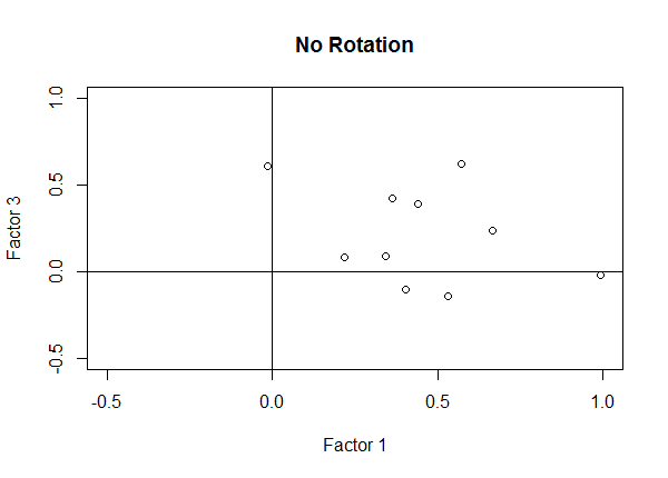
Let's fit two 4-factor models, one with no rotation and one with varimax rotation, and make a scatterplot of the first and third loadings.
Notice the scatterplot of the unrotated model has points in the "middle" of the upper-right quadrant. There are not many high or low loadings; most are moderate in size.
fa.none <- factanal(covmat = od.data, n.obs = 280, factors = 4, rotation = "none")
plot(fa.none$loadings[,1], fa.none$loadings[,3], xlim = c(-0.5, 1), ylim = c(-0.5, 1),
          xlab = "Factor 1", ylab = "Factor 3", main = "No Rotation")
abline(h = 0, v = 0)
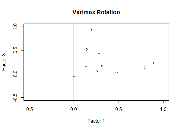
Now look at the scatterplot of the loadings with a varimax rotation. Notice the points are now clumping around axes. That is, they're high on one axis but not the other. We have more high and low loadings and fewer moderate-sized loadings, which makes for easier interpretation.
fa.varimax <- factanal(covmat = od.data, n.obs = 280, factors = 4, rotation = "varimax")
plot(fa.varimax$loadings[,1], fa.varimax$loadings[,3], xlim = c(-0.5, 1), ylim = c(-0.5, 1),
          xlab = "Factor 1", ylab = "Factor 3", main = "Varimax Rotation")
abline(h = 0, v = 0)
Factor analysis can seem overwhelming with so many estimation and rotation options along with gigantic amounts of output. (The output of the factanal() function is pretty tame compared to other programs.) However, the most important decision is number of factors. The choice of estimation method and rotation is less crucial, according to Johnson and Wichern (2007). If a factor analysis is successful, various combinations of estimations and rotations should result in the same conclusion.
On a disappointing note, Johnson and Wichern (2007) also state that the "vast majority of attempted factor analyses do not yield clear-cut results" (p. 526). There is no guarantee a factor analysis will lead to a satisfying discovery of meaningful latent factors. If you find yourself puzzling over the results of a factor analysis because it didn't seem to "work," there's a good chance you did nothing wrong and that the factor analysis simply didn't find anything interesting. A good place to start is examining the correlation matrix of your data. If there are few or no instances of high correlations, there really is no use in pursuing a factor analysis.
R session details
Analyses were conducted using the R Statistical language (version 4.5.2; R Core Team, 2025) on Windows 11 x64 (build 26100.
References
- Johnson RA and Wichern DW (2007) Applied Multivariate Statistical Analysis (6th ed). Pearson, 2007.
- Linden M (1977). “A Factor Analytic Study of Olympic Declathon Study.” Research Quarterly, 48, no. 3, 562-568.
- R Core Team (2025). R: A Language and Environment for Statistical Computing. R Foundation for Statistical Computing, Vienna, Austria. https://www.R-project.org/.
- Venables WN and Ripley BD (2002), Modern Applied Statistics with S-PLUS (4th ed). Springer.
Clay Ford
Statistical Research Consultant
University of Virginia Library
August 1, 2016
For questions or clarifications regarding this article, contact statlab@virginia.edu.
View the entire collection of UVA Library StatLab articles, or learn how to cite.