Comparing Mixed-Effect Models in R and SPSS

Occasionally we are asked to help students or faculty implement a mixed-effect model in SPSS. Our training and expertise is primarily in R, so it can be challenging to transfer and apply our knowledge to SPSS. In this article we document for posterity how to fit some basic mixed-effect models in R using the lme4 and nlme packages, and how to replicate the results in SPSS.

In this article we work with R 4.2.0, lme4 version 1.1-29, nlme version 3.1-157, and SPSS version 28.0.1.1.

To begin we fit a model in R using the sleepstudy dataset that comes with lme4. This dataset contains average reaction time per day (in milliseconds) to a psychomotor vigilance task (PVT) for subjects in a sleep deprivation study. Each subject was observed for 10 days. Of interest is how sleep-deprived subjects’ reaction times change over time.

After we load the lme4 package, we load the sleepstudy dataset into our global environment using the data() function. Once loaded we export the data as a CSV file to our working directory using write.csv(), so we can import it into SPSS.

# install.packages("lme4")
library(lme4)
data("sleepstudy")
write.csv(sleepstudy, "sleepstudy.csv", row.names = FALSE)

Here's the exported CSV file if you would like to download it: sleepstudy.csv

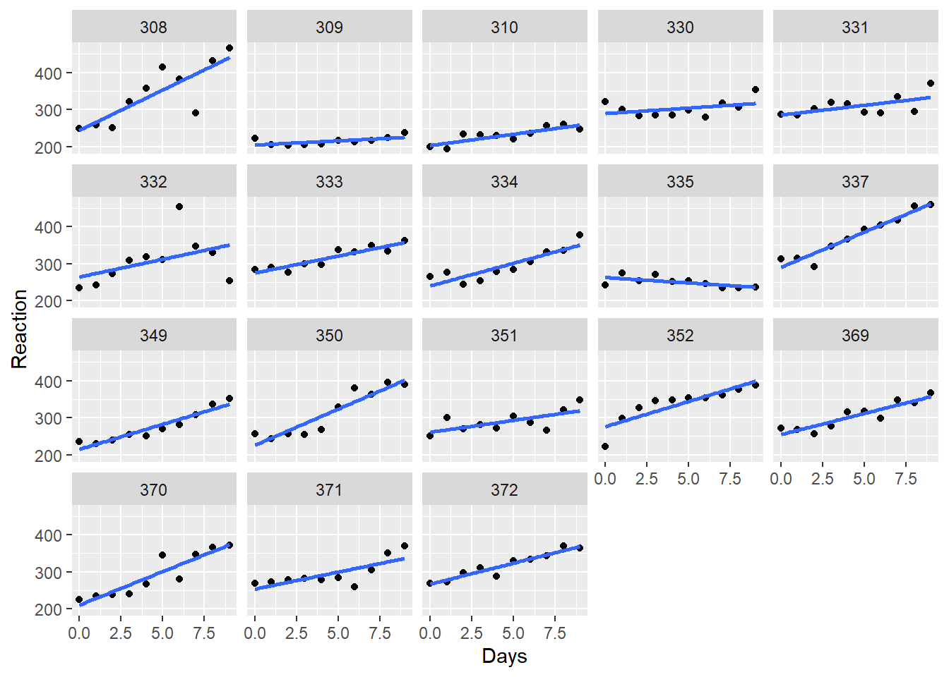
Visualizing the data with ggplot2 reveals that a linear model would seem to be suitable, but one that takes into account the random variation between subjects. It appears the subjects exert a random effect on both the intercept and slope of the fitted lines. In other words it looks like we should fit a mixed-effect model.

library(ggplot2)
ggplot(sleepstudy) +
  aes(x = Days, y = Reaction) +
  geom_point() +
  geom_smooth(method = "lm", se = FALSE) +
  facet_wrap(~Subject) 

To model Reaction as a function Days with the intercept and slope coefficients conditional on Subject, we fit the following model using lmer().

m1 <- lmer(Reaction ~ Days + (Days | Subject), sleepstudy)

The (Days | Subject) syntax says we want to model a random effect for the intercept, a random effect for the Days coefficient, and the correlation between the random effects. Random effects are variances, so we can symbolize this with the following covariance matrix, where \(\sigma^2_1\) is the intercept random effect, \(\sigma^2_2\) is the Days random effects, and \(\rho_{12}\) is the correlation between the two variances:

\[\begin{bmatrix} \sigma^2_1 & \rho_{12} \\ \rho_{12} & \sigma^2_2 \end{bmatrix} \]

Usually a covariance matrix contains covariance on the off-diagonals, not correlation. But we present it this way to conform to how lme4 summarizes random effects. Plus, correlation is simply a unitless version of covariance.

The summary output of the lme4 model lists the estimated variances/standard deviations and correlation under “Random effects”. (The corr = FALSE argument in the summary() function says to not show the correlation of fixed effects, which is not relevant to the current article.)

summary(m1, corr = FALSE)

  Linear mixed model fit by REML ['lmerMod']
  Formula: Reaction ~ Days + (Days | Subject)
     Data: sleepstudy
  
  REML criterion at convergence: 1743.6
  
  Scaled residuals: 
      Min      1Q  Median      3Q     Max 
  -3.9536 -0.4634  0.0231  0.4634  5.1793 
  
  Random effects:
   Groups   Name        Variance Std.Dev. Corr
   Subject  (Intercept) 612.10   24.741       
            Days         35.07    5.922   0.07
   Residual             654.94   25.592       
  Number of obs: 180, groups:  Subject, 18
  
  Fixed effects:
              Estimate Std. Error t value
  (Intercept)  251.405      6.825  36.838
  Days          10.467      1.546   6.771

The estimated covariance matrix for the random effects (with correlation on the off-diagonal) is:

\[\begin{bmatrix} 612.10 & 0.07 \\ 0.07 & 35.07 \end{bmatrix} \]

Now let’s replicate the same result in SPSS.

First we need to load the data. Go to File…Import Data…CSV Data, navigate to the location of the “sleepstudy.csv” file and click Open. In the Read CSV File dialog, make sure the “First line contains variables names” is checked and click OK.

Now we fit the model by going to Analyze…Mixed Models…Linear… This can be performed using SPSS syntax but we’ll show how to use the dialogs, as this seems to be how most people prefer to use SPSS (at least in our experience).

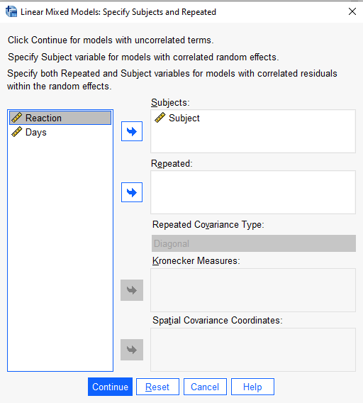
In the “Specify Subjects and Repeated” dialog, add Subject to the “Subjects:” field and click Continue. (This variable does not have to be named “Subject”; this is only a coincidence. Common names for grouping structures include “id”, “plot”, “subject_id”, and so on.)

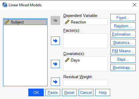
In the next dialog, “Linear Mixed Models”, add “Reaction” to the “Dependent Variable:” field and “Days” to the “Covariate(s):” field. (If we had any categorical predictors we would put them in “Factor(s)” field.)

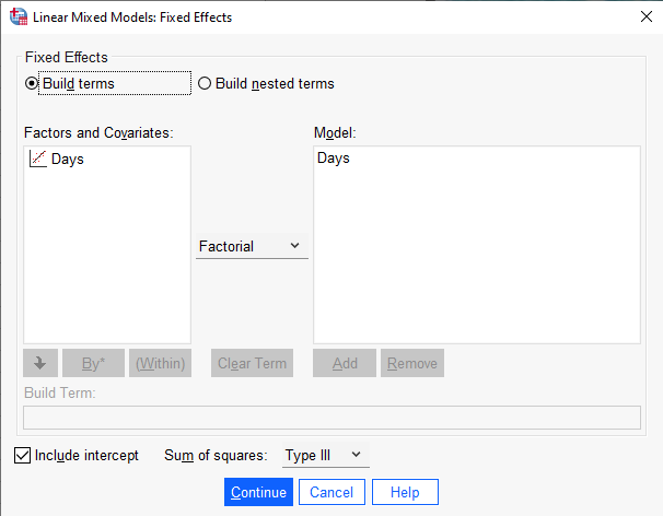
Next click the “Fixed…” button to specify our model. In this case we only have one predictor and an intercept, so we select Days under “Factors and Covariates:” and click the “Add” button. Make sure the “Include intercept” option is checked and click “Continue”. Everything else can stay the same.

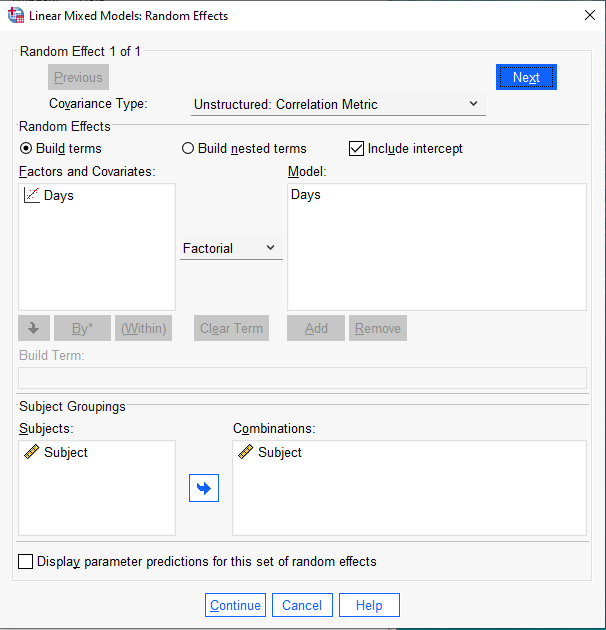
Next click the “Random…” button to specify our random effects. The first thing we need to do in this dialog is select “Unstructured: Correlation Metric” from the “Covariance Type:” pulldown. This says to use the covariance matrix we specified above. “Unstructured” means estimate all three parameters: the two variances and the covariance/correlation. We are not imposing any structure on our covariance matrix. “Correlation Metric” means return the correlation between the random effects instead of the covariance.

Then we specify which factors and covariates will have a random effect. Select Days and click “Add”. Make sure “Include intercept” is checked. Finally, under “Subject Groupings” we specify which grouping variables indicate random effects. In this case it’s Subject, so we select it, click the add arrow, and click “Continue”. Everything else can stay the same.

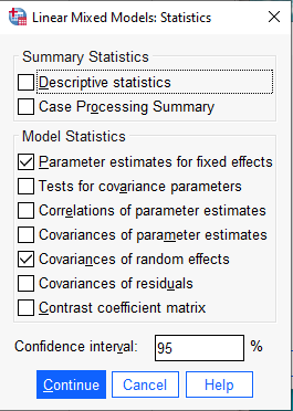
Next click the “Statistics…” button to select which statistics we want computed for our linear mixed-effect model. To keep output minimal, we select two choices:

• Parameter estimates for fixed effects
• Covariances of random effects

When done click “Continue”.

Finally we click OK to run the model. A partial listing of the output shows results equivalent to the lme4 output (within rounding error). SPSS also provides additional statistics that lme4 does not provide such as approximate p-values for the coefficient tests and standard errors for the random effects.

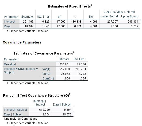
Notice in the “Estimates of Covariance Parameters” output the variances and correlation are labeled with numbers to indicate their position in the covariance matrix:

\[\begin{bmatrix} \text{Var(1)} & \text{Corr(2,1)} \\ \text{Corr(2,1)} & \text{Var(2)} \end{bmatrix} \]

This is identical to the previous covariance matrix we presented above, but with names instead of Greek symbols. SPSS also prints the covariance matrix in the next section “Random Effect Covariance Structure”, but with the estimated covariance instead of the correlation.

The estimated correlation between the random effects is quite small, about 0.07. Perhaps we could assume the correlation is 0 and fit a simpler model. This would mean imposing some structure on the covariance matrix for the random effects, as follows:

\[\begin{bmatrix} \text{Var(1)} & 0 \\ 0 & \text{Var(2)} \end{bmatrix} \]

To specify this using lmer(), we use two pipes instead of one when specifying the random effects:

# Notice the || in the random effects syntax
m2 <- lmer(Reaction ~ Days + (Days || Subject), sleepstudy)
summary(m2, corr = FALSE)

  Linear mixed model fit by REML ['lmerMod']
  Formula: Reaction ~ Days + ((1 | Subject) + (0 + Days | Subject))
     Data: sleepstudy
  
  REML criterion at convergence: 1743.7
  
  Scaled residuals: 
      Min      1Q  Median      3Q     Max 
  -3.9626 -0.4625  0.0204  0.4653  5.1860 
  
  Random effects:
   Groups    Name        Variance Std.Dev.
   Subject   (Intercept) 627.57   25.051  
   Subject.1 Days         35.86    5.988  
   Residual              653.58   25.565  
  Number of obs: 180, groups:  Subject, 18
  
  Fixed effects:
              Estimate Std. Error t value
  (Intercept)  251.405      6.885  36.513
  Days          10.467      1.560   6.712

Notice there is no estimated correlation in the “Random effects” section. That’s because we constrained it to be 0.

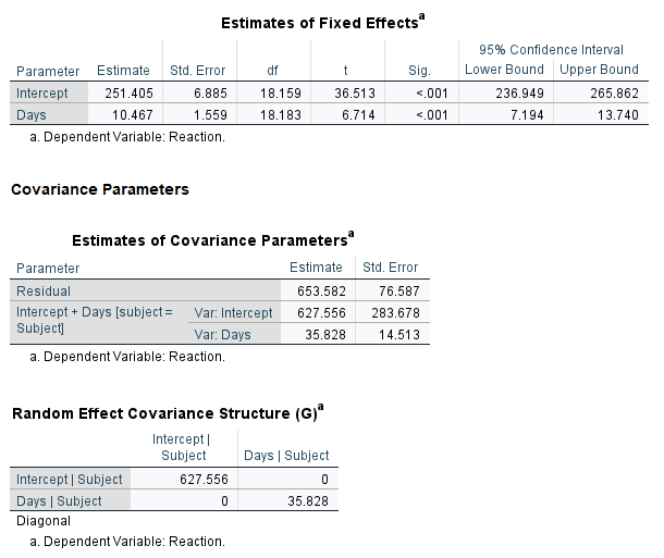
To replicate this model in SPSS, we follow all the same steps above except we select “Diagonal” in the “Covariance Type:” pulldown in the Random Effects dialog.

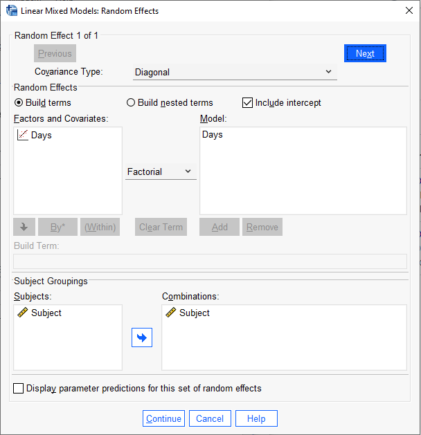
The SPSS output for the random effects is basically the same as the lme4 output with some mild discrepancies in the decimals. This is likely due to minor differences in the default settings of the optimization routines. Notice the Random Effect Covariance Structure shows a 0 on the off-diagonal.

A further constraint on the random effect covariance matrix would be to assume both variances are equal.

\[\begin{bmatrix} \text{Var} & 0 \\ 0 & \text{Var} \end{bmatrix} \]

In this case there is only one variance parameter to estimate. Based on the estimated random effects we’ve seen so far, this seems like a far-fetched assumption. There is far more variability between subject reaction times on day 0 (the intercept) than there is between their estimated slopes. However for the sake of completeness we’ll demonstrate how to fit this covariance structure.

Unfortunately, the lmer() function in the lme4 package does not provide facilities for this type of structure. To entertain this model we turn to the nlme package and the function lme(). To specify random effects in the lme() function we use the random argument. To specify that we want to estimate one common variance parameter for both random effects, we use the pdIdent() function. The syntax is a little awkward if you’re accustomed to lme4. We need to set Subject = pdIdent(~ Days) and nest in a list. The summary output shows one estimate of standard deviation (the square root of variance) for both Intercept and Days random effects: 8.89.

# no need to install, comes with R
library(nlme)
m3 <- lme(Reaction ~ Days, random = list(Subject = pdIdent(~ Days)), 
          data = sleepstudy)
summary(m3)

  Linear mixed-effects model fit by REML
    Data: sleepstudy 
        AIC      BIC    logLik
    1767.15 1779.877 -879.5749
  
  Random effects:
   Formula: ~Days | Subject
   Structure: Multiple of an Identity
          (Intercept)     Days Residual
  StdDev:    8.898743 8.898743 27.37447
  
  Fixed effects:  Reaction ~ Days 
                  Value Std.Error  DF  t-value p-value
  (Intercept) 251.40510  4.333705 161 58.01158       0
  Days         10.46729  2.214483 161  4.72674       0
   Correlation: 
       (Intr)
  Days -0.237
  
  Standardized Within-Group Residuals:
          Min          Q1         Med          Q3         Max 
  -3.77675971 -0.54676522  0.03842765  0.57370461  4.86391328 
  
  Number of Observations: 180
  Number of Groups: 18

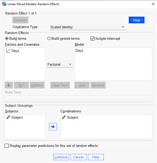
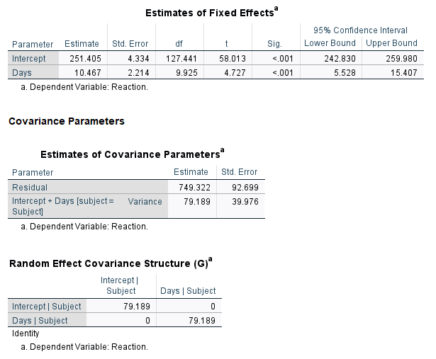
To replicate this model in SPSS, we follow all the same steps above except we select “Scaled Identity” in the “Covariance Type:” pulldown in the Random Effects dialog.

The SPSS output for the random effects shows one variance, 79.189, instead of one standard deviation. You can square the nlme output or take the square root of the SPSS output to see they’re the same.

Which model is better? One way to assess this is to compare information criteria such as AIC or BIC. We leave it to the interested reader to verify that m2 is probably the preferable model.

There is much more to mixed-effect modeling in lme4, nlme and SPSS. In this article we simply discussed modeling the covariance structure of random effects for a basic mixed-effect model, and showed how to implement the same models in R and SPSS. We hope anyone obligated to move from R to SPSS, or vice versa, will find this helpful.

References

• Bates D, Maechler M, Bolker B, Walker S (2015). Fitting Linear Mixed-Effects Models Using lme4. Journal of Statistical Software, 67(1), 1-48. doi:10.18637/jss.v067.i01.
• Belenky G, et al (2003) Patterns of performance degradation and restoration during sleep restriction and subsequent recovery: a sleep dose-response study. Journal of Sleep Research 12, 1–12.
• IBM Corp. Released 2021. IBM SPSS Statistics for Windows, Version 28.0.0.1. Armonk, NY: IBM Corp
• Pinheiro J, Bates D, R Core Team (2022). nlme: Linear and Nonlinear Mixed Effects Models. R package version 3.1-157, https://CRAN.R-project.org/package=nlme.
• R Core Team (2022). R: A language and environment for statistical computing. R Foundation for Statistical Computing, Vienna, Austria. URL https://www.R-project.org/.
• Wickham, H (2016). ggplot2: Elegant Graphics for Data Analysis. Springer-Verlag New York.

Clay Ford
Statistical Research Consultant
University of Virginia Library
May 03, 2022